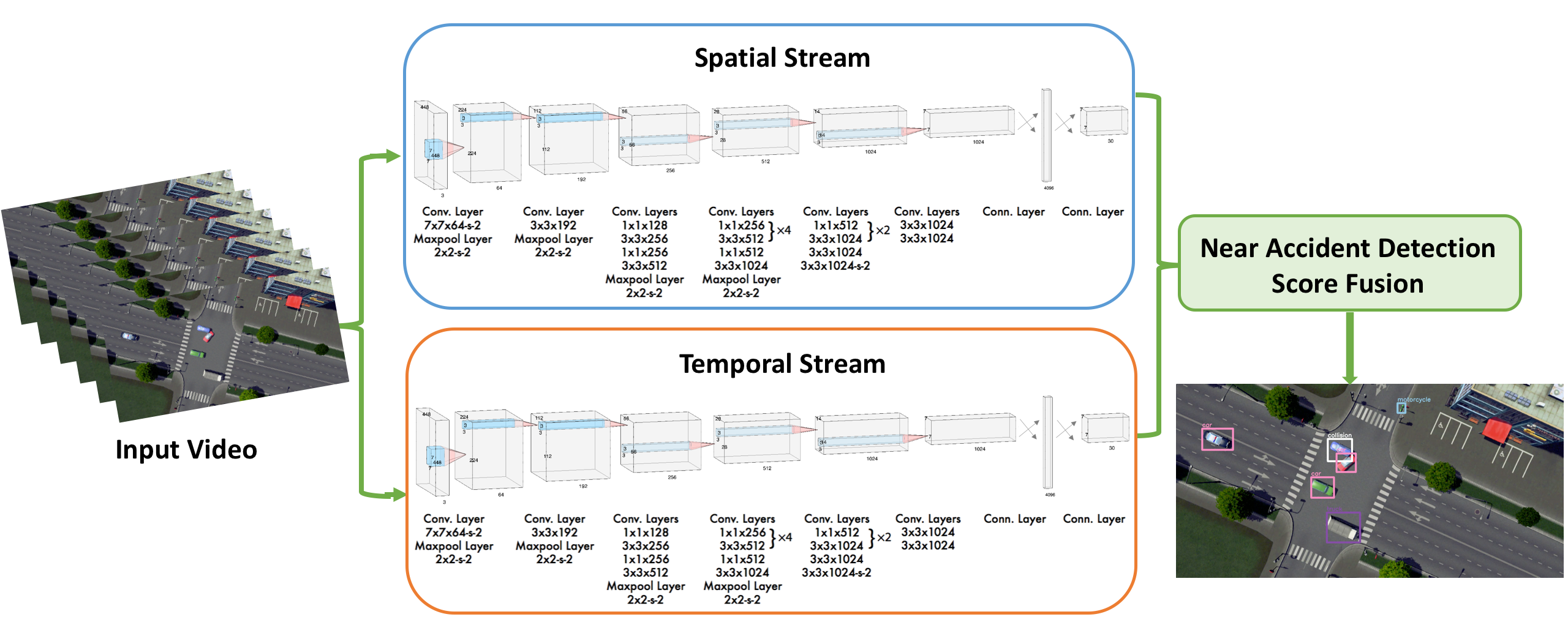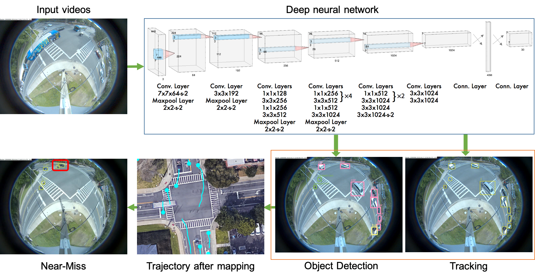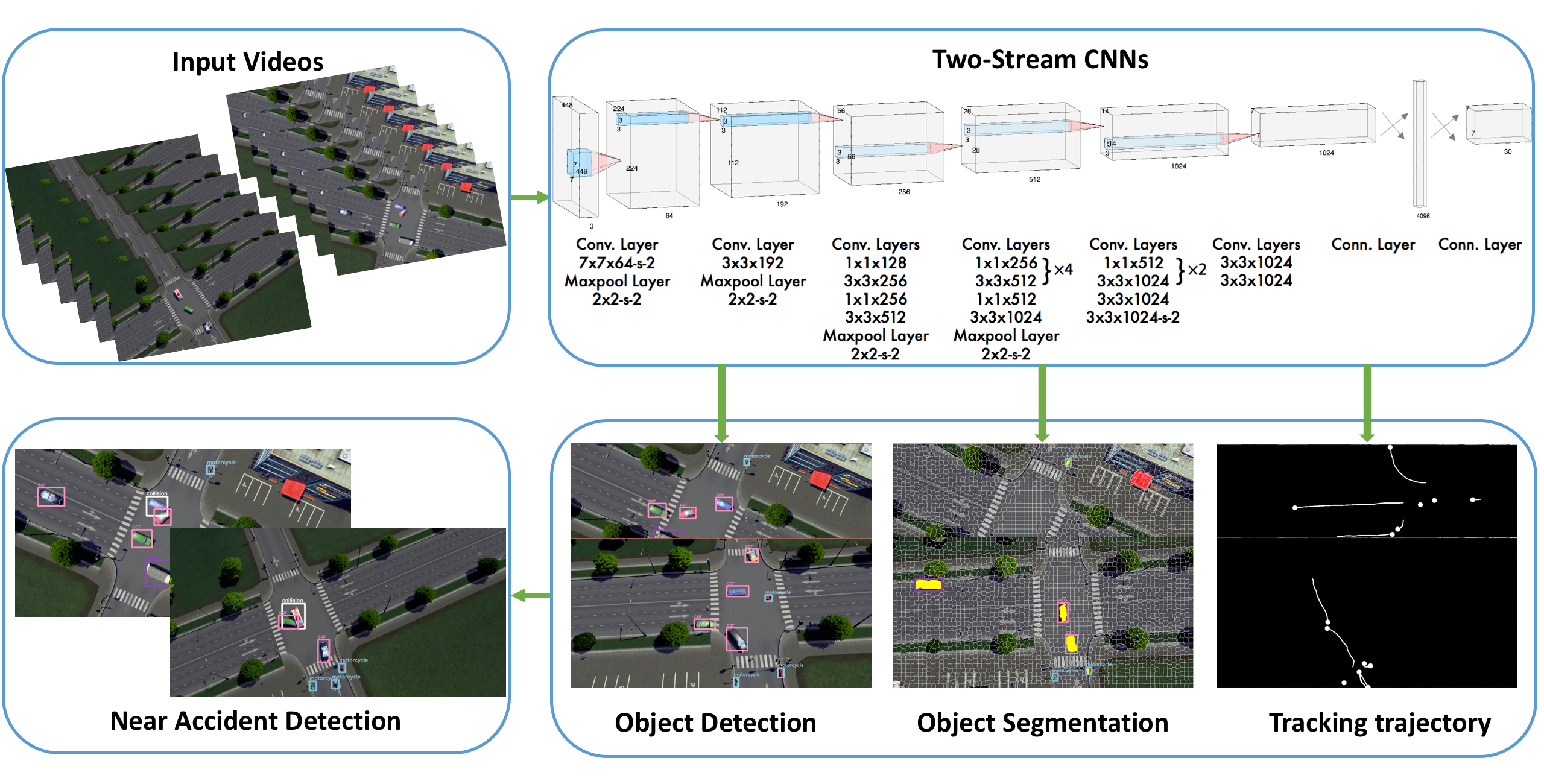
| Figure 2.1.: | The overall pipeline of our two-stream convolutional neural networks for near-miss detection. |
| Xiaohui Huang |
| Aotian Wu |
| Ke Chen |
| Anand Rangarajan |
| Sanjay Ranka |
This book is intended for pedagogical purposes and the authors have taken care to provide details based on their experience. However, the authors do not guarantee that the material in this book is accurate or will be effective in practice, nor are they responsible for any statement, material or formula that may have negative consequences, injuries, death etc. to the readers or the users of the book.
Rapid urbanization worldwide, the growing volume of vehicular traffic, and the increasing complexity of roadway networks have led to congestion, traffic jams, and traffic incidents [1, 2]], which negatively affect productivity [3], the well-being of the society [4], and the environment [5]. Therefore, keeping traffic flowing smoothly and safely is essential for traffic engineers.
Significant advances in electronics, sensing, computing, data storage, and communications technologies in intelligent transportation systems (ITS) [6, 7] have led to some commonly seen aspects of ITS [8] which include:
This book presents algorithms and methods for using video analytics to process traffic data. Edge-based real-time machine learning (ML) techniques and video stream processing have several advantages. (1) There is no need to store copious amounts of video (a few minutes typically suffice for edge-based processing), thus addressing concerns of public agencies who do not want person-identifiable information to be stored for reasons of citizen privacy and legality. (2) The processing of the video stream at the edge will allow for the use of low bandwidth communication using wireline and wireless networks to a central system such as a cloud, resulting in a compressed and holistic picture of the entire city. (3) The real-time processing enables a wide variety of novel transportation applications at the intersection, street, and system levels that were not possible hitherto, significantly impacting safety and mobility.
The existing monitoring systems and decision-making for this purpose have several limitations:
In Section 1.2, we will describe the data sources from which we collect and store loop recorder data and video data. Section 1.3 summarizes the rest of the chapters in the book.
| Table 1.1.: | Raw event logs from signal controllers. Most modern controllers generate these data at a frequency of 10 Hz. |
| SignalID | Timestamp | EventCode | EventParam |
| 1490 | 2018-08-01 00:00:00.000100 | 82 | 3 |
| 1490 | 2018-08-01 00:00:00.000300 | 82 | 8 |
| 1490 | 2018-08-01 00:00:00.000300 | 0 | 2 |
| 1490 | 2018-08-01 00:00:00.000300 | 0 | 6 |
| 1490 | 2018-08-01 00:00:00.000300 | 46 | 1 |
| 1490 | 2018-08-01 00:00:00.000300 | 46 | 2 |
| 1490 | 2018-08-01 00:00:00.000300 | 46 | 3 |
Signal controllers, based on the latest Advanced Transportation Controller (ATC)1 standards, are capable of recording signal events (e.g., vehicle arrival and departure events) at a high data rate (10 Hz). The different attributes in the data include intersection identifier, timestamp, and EventCode and EventParam. The accompanying metadata describes what different EventCode and EventParam indicate. For instance, EventCode 82 denotes vehicle arrival, and the corresponding EventParam represents the detector channel that captured the event. The other necessary metadata is the detector channel to lane/phase mapping, which helps to identify the lane corresponding to a specific detector channel. Different performance measures of interest, such as arrivals on red, arrivals on green, or demand-based split failures, can be derived on a granular level (cycle-by-cycle) using these data.
We process videos captured by fisheye cameras installed at intersections. A fisheye (bell) camera has an ultrawide angle lens, resulting in a wide panoramic view of the nonrectilinear image. Acquiring locations with a fisheye camera is advantageous because it can obtain a complete picture of the entire intersection.
The fisheye intersection videos are more challenging than videos collected by surveillance cameras for reasons including fisheye distortion, multiple object types (pedestrians and vehicles), and diverse lighting conditions. We annotated the spatial location (bounding boxes) and temporal location (frames) for each object and their vehicle class in videos for each intersection to generate ground truth for object detection, tracking, and near-miss detection.
The chapters are organized as follows. In Chapter 2, we propose an integrated two-stream convolutional network architecture that performs real-time detection, tracking, and near-miss detection of road users in traffic video data. The two-stream model consists of a spatial stream network for object detection and a temporal stream network to leverage motion features for multiple object tracking. We detect near-misses by incorporating appearance features and motion features from these two networks. Further, we demonstrate that our approaches can be executed in real-time and at a frame rate higher than the video frame rate on various videos.
In Chapter 3, we introduce trajectory clustering and anomaly detection algorithms. We develop real-time or near real-time algorithms for detecting near-misses for intersection video collected using fisheye cameras. We propose a novel method consisting of the following steps: (1) extracting objects and multiple object tracking features using convolutional neural networks; (2) densely mapping object coordinates to an overhead map; and (3) learning to detect near-misses by new distance measures and temporal motion. The experiments demonstrate the effectiveness of our approach with a real-time performance at 40 fps and high specificity.
Chapter 4 presents an end-to-end software pipeline for processing traffic videos and running a safety analysis based on surrogate safety measures. As a part of road safety initiatives, surrogate road safety approaches have gained popularity due to the rapid advancement of video collection and processing technologies. We developed algorithms and software to determine trajectory movement and phases that, when combined with signal timing data, enable us to perform accurate event detection and categorization regarding the type of conflict for both pedestrian-vehicle and vehicle-vehicle interactions. Using this information, we introduce a new surrogate safety measure, “severe event,” which is quantified by multiple existing metrics such as time-to-collision (TTC) and post-encroachment time (PET) as recorded in the event, deceleration, and speed. We present an efficient multistage event-filtering approach followed by a multi-attribute decision tree algorithm that prunes the extensive set of conflicting interactions to a robust set of severe events. The above pipeline was used to process traffic videos from several intersections in multiple cities to measure and compare pedestrian and vehicle safety. Detailed experimental results are presented to demonstrate the effectiveness of this pipeline.
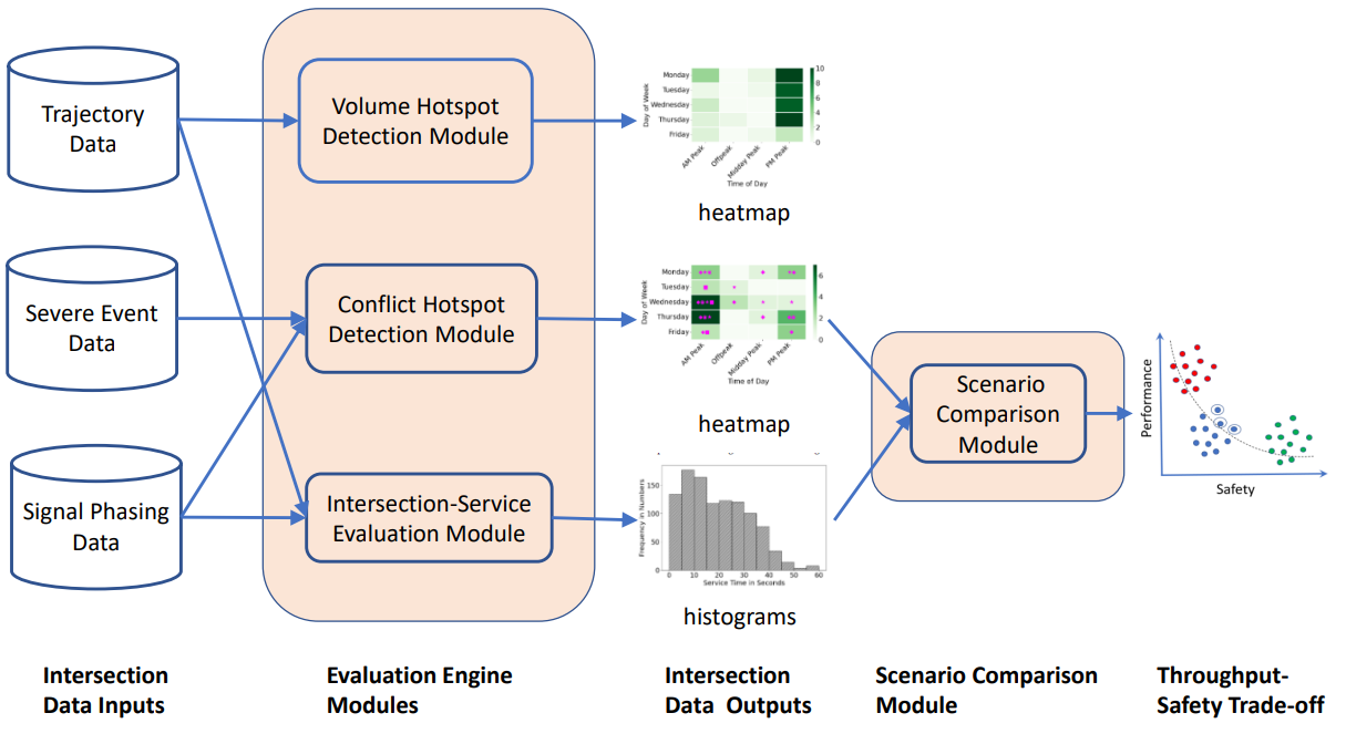
Chapter 5 illustrates cutting-edge methods by which conflict hotspots can be detected in various situations and conditions. Both pedestrian-vehicle and vehicle-vehicle conflict hotspots can be discovered, and we present an original technique for including more information in the graphs with shapes. Conflict hotspot detection, volume hotspot detection, and intersection-service evaluation allow us to comprehensively understand the safety and performance issues and test countermeasures. The selection of appropriate countermeasures is demonstrated by extensive analysis and discussion of two intersections in Gainesville, Florida, USA. Just as important is the evaluation of the efficacy of countermeasures. This chapter advocates for selection from a menu of countermeasures at the municipal level, with safety as the top priority. Performance is also considered, and we present a novel concept of a performance-safety trade-off at intersections.
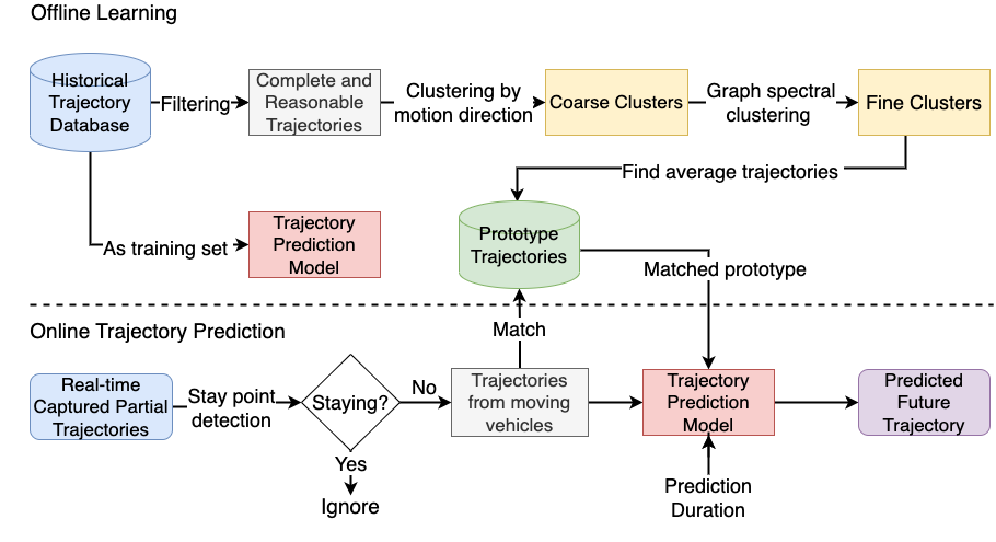
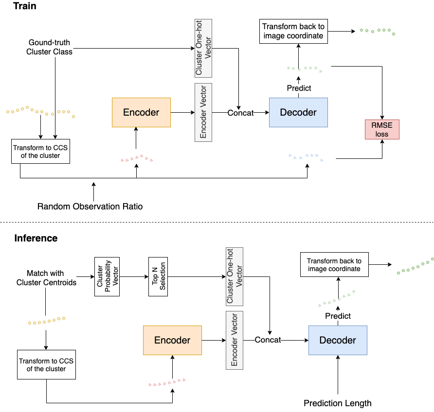
In Chapter 6, we propose to perform trajectory prediction using surveillance camera images. As vehicle-to-infrastructure (V2I) technology enables low-latency wireless communication, warnings from our prediction algorithm can be sent to vehicles in real-time. Our approach consists of an offline learning phase and an online prediction phase. The offline phase learns common motion patterns from clustering, finds prototype trajectories for each cluster, and updates the prediction model. The online phase predicts the future trajectories for incoming vehicles, assuming they follow one of the motion patterns learned from the offline phase. We adopted a long short-term memory encoder-decoder (LSTM-ED) model for trajectory prediction. We also explored using a curvilinear coordinate system (CCS) which utilizes the learned prototype and simplifies the trajectory representation. Our model is also able to handle noisy data and variable-length trajectories. Our proposed approach outperforms the baseline Gaussian process (GP) model and shows sufficient reliability when evaluated on collected intersection data.
In Chapter 7, we propose a methodology for travel-time estimation of traffic flow, an important problem with critical implications for traffic congestion analysis. We developed techniques for using intersection videos to identify vehicle trajectories across multiple cameras and analyze corridor travel time. Our approach consists of (1) multi-object single-camera tracking, (2) vehicle re-identification among different cameras, (3) multi-object multi-camera tracking, and (4) travel-time estimation. We evaluated the proposed framework on real intersections in Florida with pan and fisheye cameras. The experimental results demonstrate the viability and effectiveness of our method.
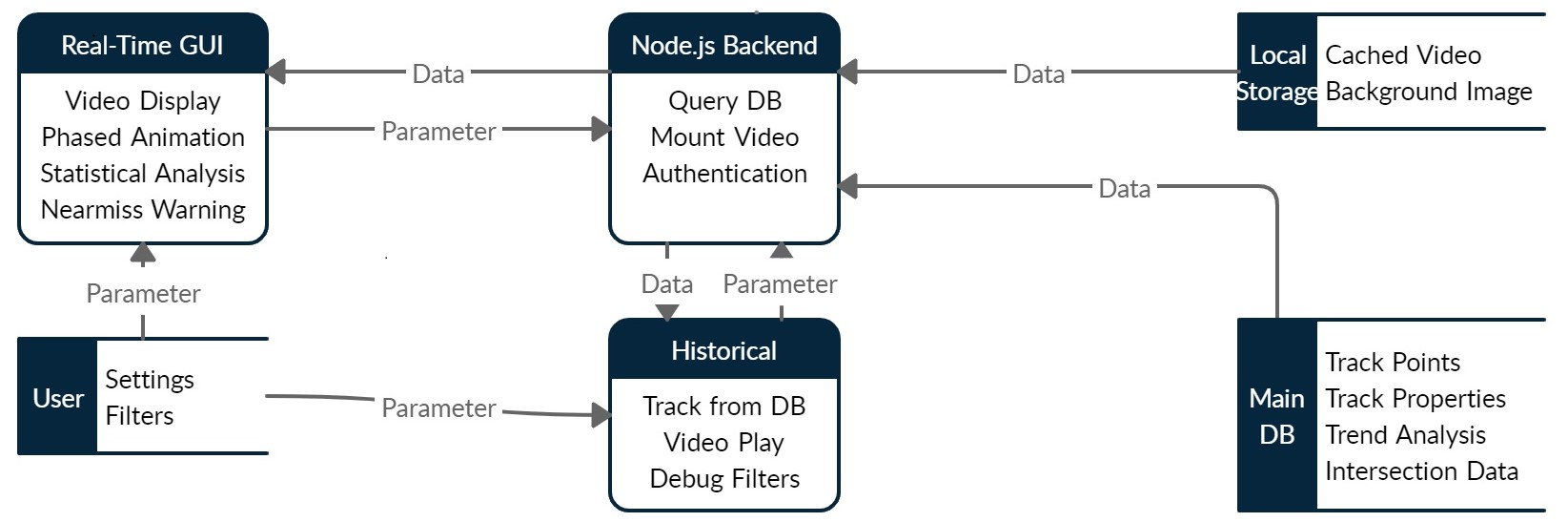
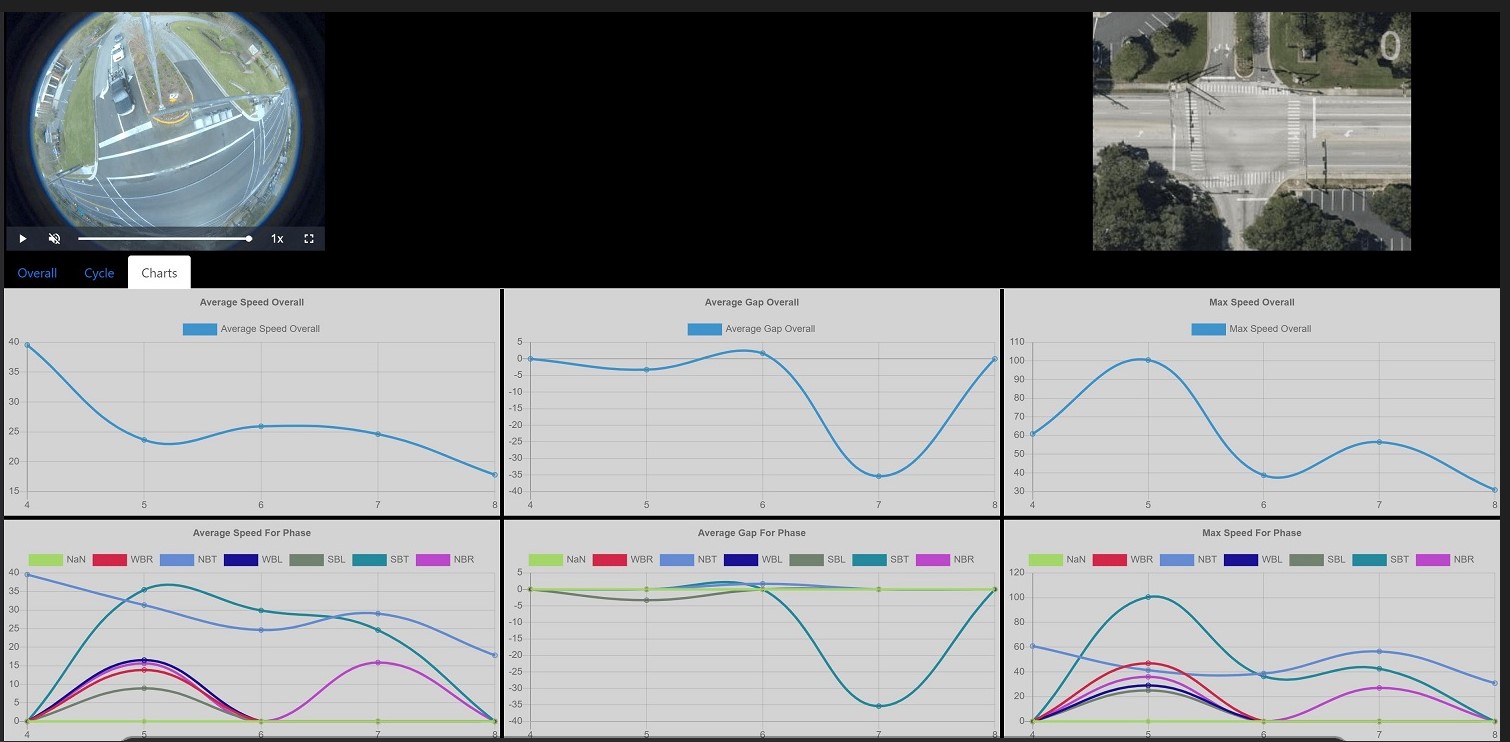
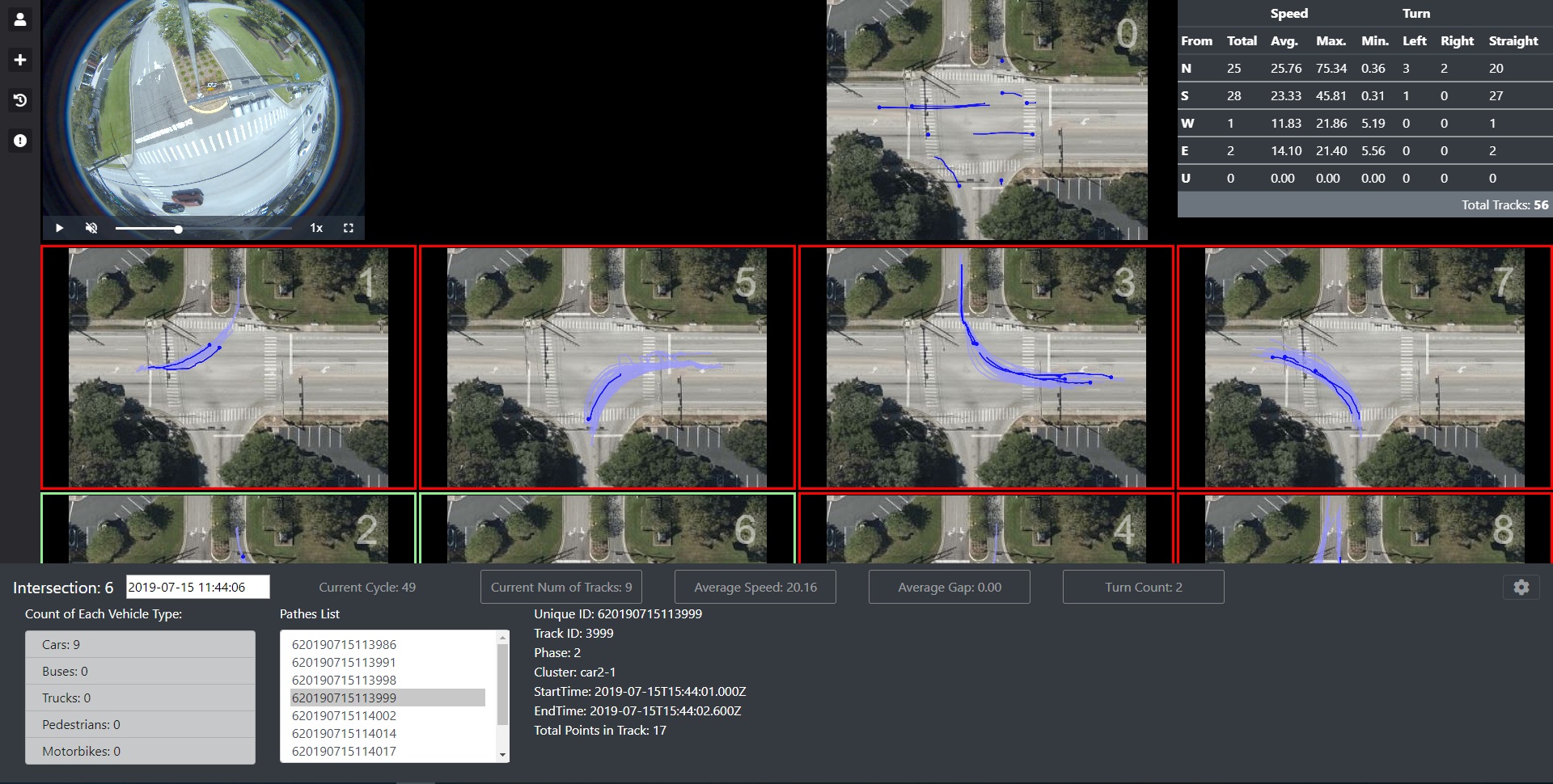
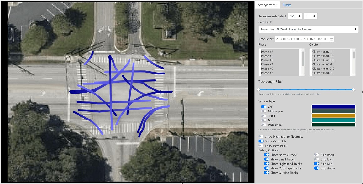
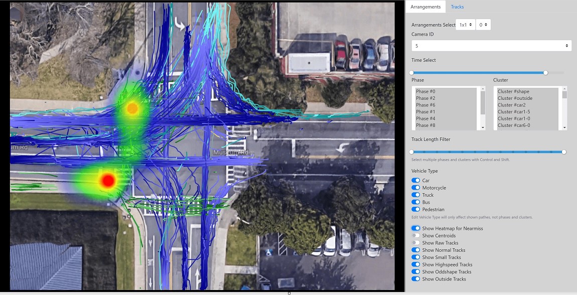
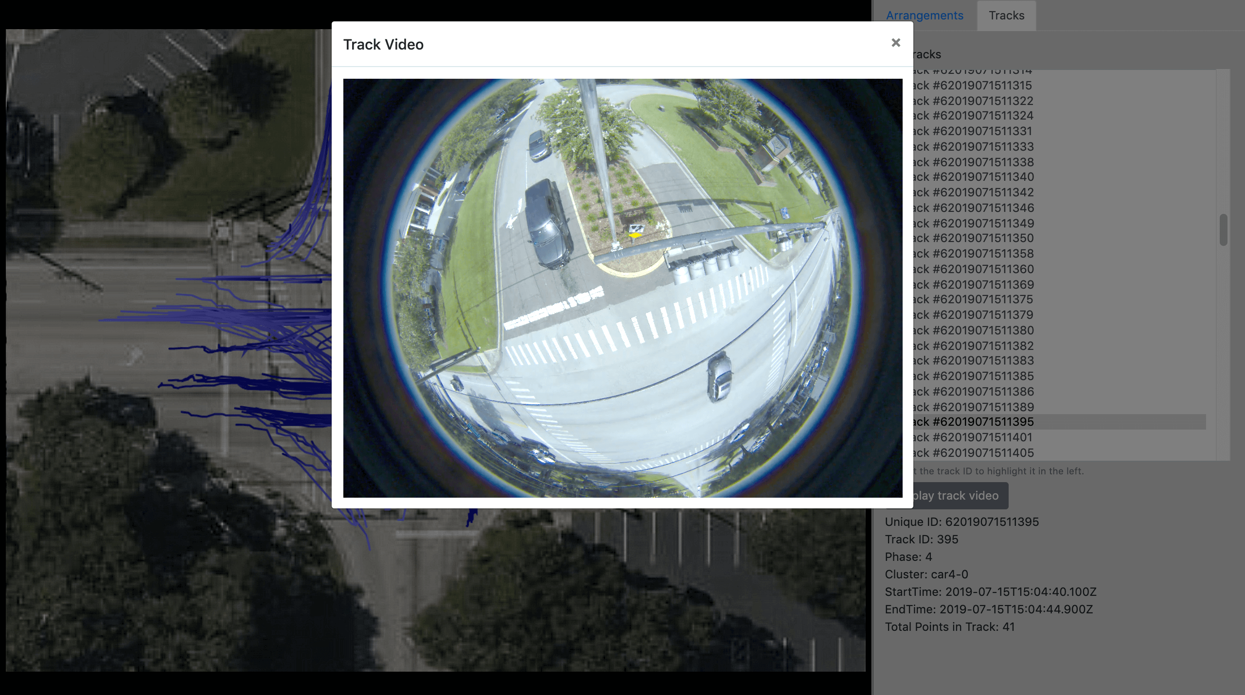
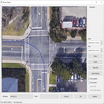
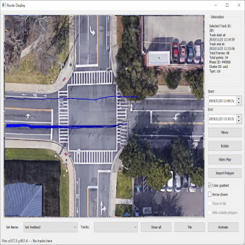
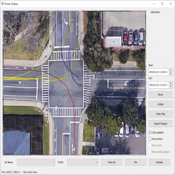
In Chapter 8, we present a visual analytics framework that traffic engineers may use to analyze the events and performance at an intersection. The tool ingests streaming videos collected from a fisheye camera, cleans the data, and runs analytics. The tool presented here has two modes: streaming and historical modes. The streaming mode may be used to analyze data close to real-time with a latency set by the user. In the historical mode, the user can run a variety of trend analyses on historical data.
In Chapter 9, we summarize the contributions of the present work.
The rapid changes in the growth of exploitable and, in many cases, open data can mitigate traffic congestion and improve safety. Despite significant advances in vehicle technology, traffic engineering practices, and analytics based on crash data, the number of traffic crashes and fatalities is still too many. Many drivers are frustrated due to prolonged (potentially preventable) intersection delays. Using video or light detection and ranging (LiDAR) processing, big data analytics, artificial intelligence, and machine learning can profoundly improve the ability to address these challenges. Collecting and exploiting large datasets are familiar to the transportation sector. However, the confluence of ubiquitous digital devices and sensors, significantly lower hardware costs for computing and storage, enhanced sensing and communication technologies, and open-source analytics solutions have enabled novel applications. The latter may involve insights into otherwise unobserved patterns that positively influence individuals and society.
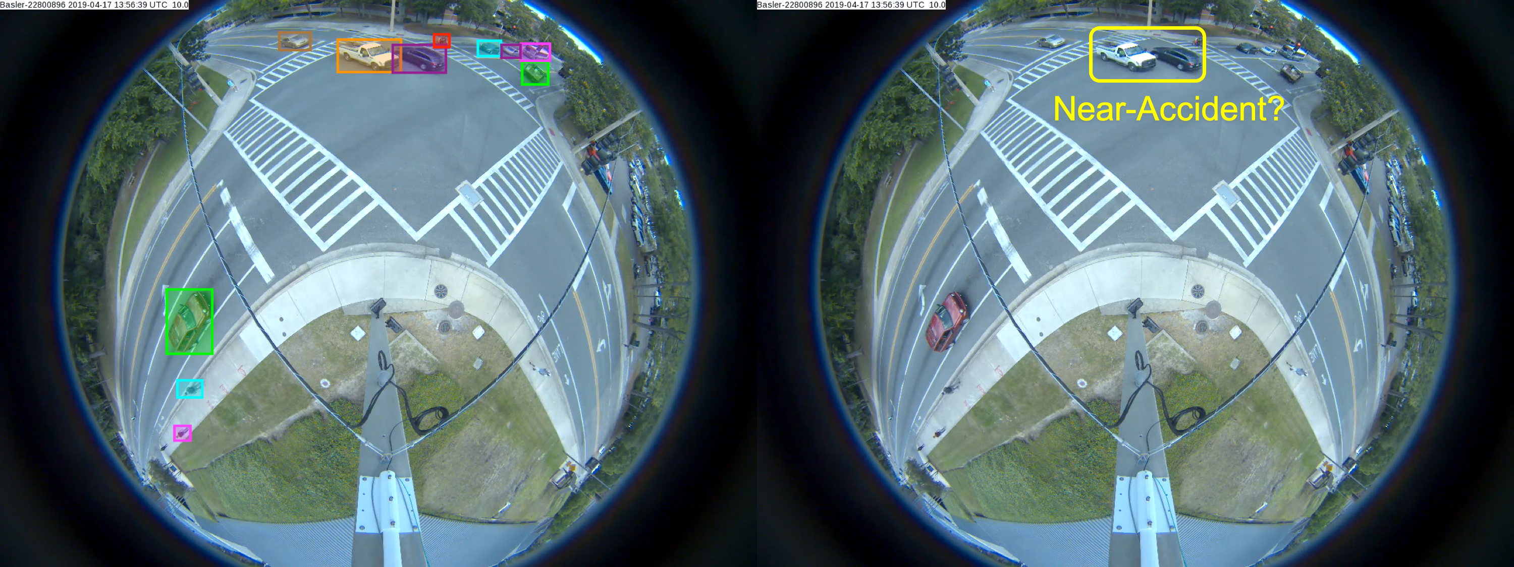
The technologies of artificial intelligence (AI) and the Internet of Things (IoT) are ushering in a new promising era of “smart cities” where billions of people around the world can improve the quality of their lives in aspects of transportation, security, information, communications, etc. One example of data-centric AI solutions is computer vision technologies that enable vision-based intelligence for edge devices across multiple architectures. Sensor data from smart devices or video cameras can be analyzed immediately to provide real-time analysis for intelligent transportation systems (ITS). At traffic intersections, there is a greater volume of road users (pedestrians and vehicles), traffic movement, dynamic traffic events, near-accidents, etc. It is a critically important application to enable global monitoring of traffic flow, local analysis of road users, and automatic near-miss detection.
As a new technology, vision-based intelligence has many applications in traffic surveillance and management [9, 10, 11, 12, 13, 14]. Many research works have focused on traffic data acquisition with aerial videos [15, 16]; the aerial view provides better perspectives to cover a large area and focus resources for surveillance tasks. Unmanned aerial vehicles (UAVs) and omnidirectional cameras can acquire helpful aerial videos for traffic surveillance, especially at intersections, with a broader perspective of the traffic scene and the advantage of being mobile and spatiotemporal. A recent trend in vision-based intelligence is to apply computer vision technologies to these acquired intersection aerial videos [17, 18] and process them at the edge across multiple ITS architectures.
Object detection and multiple object tracking are widely used applications in transportation, and real-time solutions are significant, especially for the emerging area of big transportation data. A near-miss is an event that has the potential to develop into a collision between two vehicles or between a vehicle and a pedestrian or bicyclist. These events are important to monitor and analyze to prevent crashes in the future. They are also a proxy for potential timing and design issues at the intersection. Camera-monitored intersections produce video data in gigabytes per camera per day. Analyzing thousands of trajectories collected per hour at an intersection from different sources to identify near-miss events quickly becomes challenging, given the amount of data to be examined and the relatively rare occurrence of such events.
In this work, we investigate using traffic video data for near-miss detection. However, to the best of our knowledge, a unified system that performs real-time detection and tracking of road users and near-miss detection for aerial videos is not available. Therefore, we have collected video datasets and presented a real-time deep learning-based method to tackle these problems.
Generally, a vision-based surveillance tool for ITS should meet several requirements: (1) segment vehicles from their surroundings (including other road objects and the background) to detect all road objects (still or moving); (2) classify detected vehicles into categories: cars, buses, trucks, motorbikes, etc.; (3) extract spatial and temporal features (motion, velocity, and trajectory) to enable more specific tasks, including vehicle tracking, trajectory analysis, near-miss detection, anomaly detection, etc.; (4) function under various traffic conditions and lighting conditions; and (5) operate in real-time. Over the decades, although increasing research on vision-based systems for traffic surveillance has been proposed, many of the criteria listed above still need to be met. Early solutions [19] do not identify individual vehicles as unique targets and progressively track their movements. Methods have been proposed to address individual vehicle detection and vehicle tracking problems [20, 21, 9] with tracking strategies and optical flow deployment. Compared to traditional hand-crafted features, deep learning methods [22, 23, 24, 25, 26, 27] in object detection have illustrated the robustness of specialization of the generic detector to a specific scene. Recently, automatic traffic accident detection has become an important topic. Before detecting accident events [28, 12, 29, 30, 31], one typical approach is to apply object detection or tracking methods using a histogram of flow gradient (HFG), hidden Markov model (HMM) or Gaussian mixture model (GMM). Other approaches [32, 33, 34, 35, 36, 37, 38, 39, 40] use low-level features (e.g., motion features) to demonstrate better robustness. Neural networks have also been employed for automatic accident detection [41, 42, 43, 44].
| Figure 2.1.: | The overall pipeline of our two-stream convolutional neural networks for near-miss detection. |
The overall pipeline of our method is depicted in Figure 2.1. The organization of this chapter is as follows. Section 2.2 describes the background of convolutional neural networks, object detection, and multiple object tracking methods. Section 2.3 describes our method’s overall architecture, methodologies, and implementation. This is followed in Section 2.4 by introducing our traffic near-accident detection dataset (TNAD) and presenting a comprehensive evaluation of our approach and other state-of-the-art near-accident detection methods, both qualitatively and quantitatively. Section 2.5 summarizes our contributions and discusses future work’s scope.
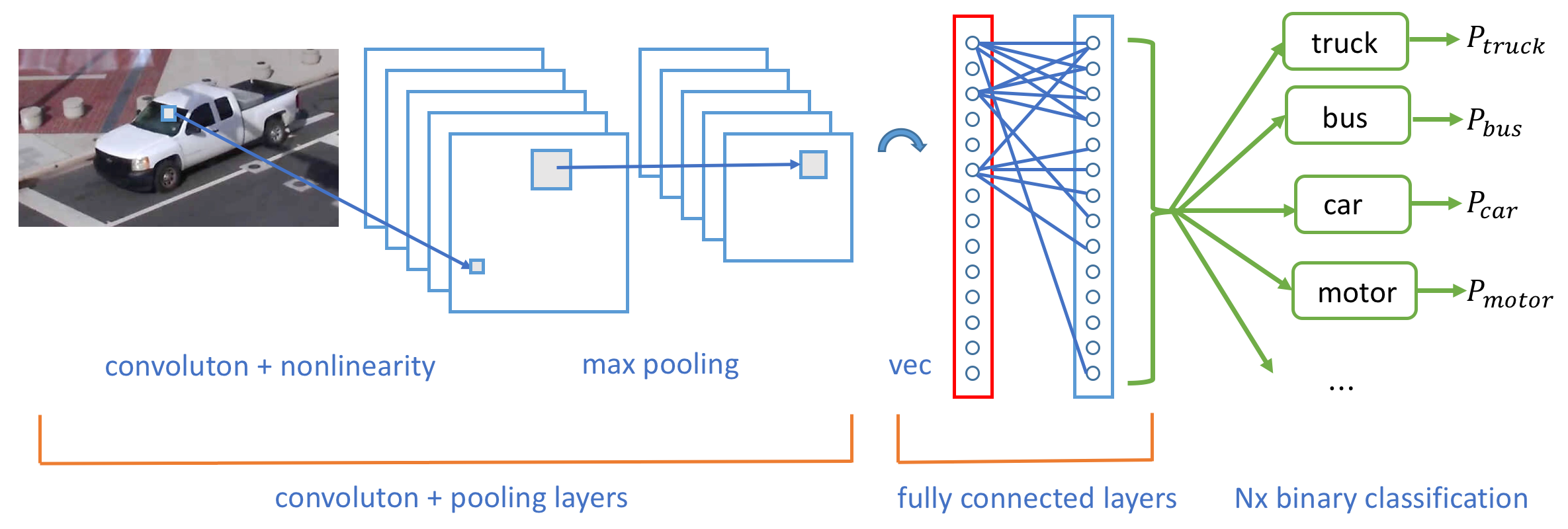
CNNs have shown strong capabilities in representing objects, thereby boosting the performance of numerous vision tasks, especially compared to traditional features [45]. A CNN is a class of deep neural networks which is widely applied in image analysis and computer vision. A standard CNN usually consists of both the input layer and the output layer, as well as multiple hidden layers (e.g., convolutional layers, fully connected layers, pooling layers), as shown in Figure 2.2. The input to a convolutional layer is an original image X. We denote the feature map of the i-th convolutional layer as Hi, and H0 = X. Then Hi can be described as
 | (2.1) |
where W i is the weight for the i-th convolutional kernel for the i � 1-th image or feature map and � is the convolution operation. The output of the convolution operation includes a bias, bi. Then, the feature map for the i-th layer can be computed by applying a standard nonlinear activation function. We briefly describe a 32 � 32 RGB image with a simple ConvNet for CIFAR-10 image classification [46]:
In this way, CNNs transform the original image into multiple high-level feature representations layer by layer, obtaining class-specific outputs or scores.
The real-time You Only Look Once (YOLO) detector, proposed in [24], is an end-to-end state-of-the-art deep learning approach without using region proposals. The pipeline of YOLO [24] is relatively straightforward: Given an input image, YOLO [24] passes it through the neural network only once, as its name implies (You Only Look Once), and outputs the detected bounding boxes and class probabilities in prediction. Figure 2.4 demonstrates the detection model and system of YOLO [24]. YOLO [24] is orders of magnitude faster (45 frames per second) than other object detection approaches, which means it can process streaming video in real-time. Compared to other systems, it also achieves a higher mean average precision. In this work, we leverage the extension of YOLO [24], Darknet-19, a classification model used as the basis of YOLOv2 [47]. Darknet-19 [47] consists of 19 convolutional layers and five max-pooling layers, where batch normalization is utilized to stabilize training, speed up convergence, and regularize the model [48].
SORT [49] is a simple, popular, fast multiple object tracking (MOT) algorithms. The core idea combines Kalman filtering [50] and frame-by-frame data association. The data association is implemented with the Hungarian method [51] by measuring the bounding box overlap. With this rudimentary combination, SORT [49] achieves a state-of-the-art performance compared to other online trackers. Moreover, due to its simplicity, SORT [49] can update at a rate of 260 Hz on a single machine, which is over 20 times faster than other state-of-the-art trackers.
DeepSORT [52] is an extension of SORT [49]. DeepSORT integrates appearance information to improve the performance of SORT [49] by adding one pre-trained association metric. DeepSORT [52] helps solve many identity-switching problems in SORT [49], and it can track occluded objects in a longer term. The measurement-to-track association is established in visual appearance space during the online application, using nearest-neighbor queries.
This section presents our computer vision-based two-stream architecture for real-time near-miss detection. The architecture is primarily driven by real-time object detection and multiple object tracking (MOT). The goal of near-accident detection is to detect likely collision scenarios across video frames and report these near-miss records. Because videos have spatial and temporal components, we divide our framework into a two-stream architecture, as shown in Figure 2.3. The spatial aspect comprises individual frame appearance information about scenes and objects. The temporal element comprises motion information of objects. For the spatial stream convolutional neural network we utilize a standard convolutional network designed for state-of-the-art object detection [24] to detect individual vehicles and mark near-miss regions at the single-frame level. The temporal stream network leverages object candidates from object detection CNNs and integrate their appearance information with a fast MOT method to extract motion features and compute trajectories. When two trajectories of individual objects intersect or come closer than a certain threshold (whose estimation is described below), we label the region covering the two entities as a high probability near-miss area. Finally, we take the average near-miss likelihood of both the spatial and temporal stream networks and report the near-miss record.
Each stream is implemented using a deep convolutional neural network in our framework. Near-accident scores are combined by averaging. Because our spatial stream ConvNet is essentially an object detection architecture, we base it on recent advances in object detectionessentially the YOLO detector [24]—and pre-train the network from scratch on our dataset containing multiscale drone, fisheye, and simulation videos. As most of our videos have traffic scenes with vehicles and movement captured in a top-down view, we specify different vehicle classes such as motorbike, car, bus, and truck as object classes for training the detector. Additionally, near-misses or collisions can be detected from single still frames or stopped vehicles associated with an accident, even at the beginning of a video. Therefore, we train our detector to localize these likely near-miss scenarios. Since static appearance is a valuable cue, the spatial stream network performs object detection by only operating on individual video frames.
The spatial stream network regresses the bounding boxes and predicts the class probabilities associated with these boxes using a simple end-to-end convolutional network. It first splits the image into a S �S grid. For each grid cell,
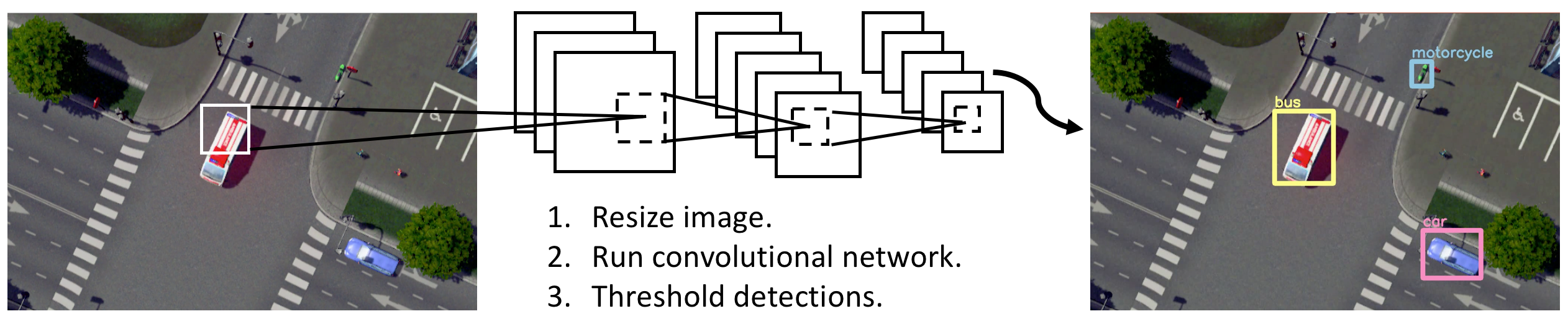
| Figure 2.4.: | Object detection pipeline of our spatial stream [24]: (1) resizes the input video frame, (2) runs convolutional network on the frame, and (3) thresholds the resulting detection by the model’s confidence. |
For each bounding box, the CNN outputs a class probability and offset values for the bounding box. Then, it selects bounding boxes that have the class probability above a threshold value and uses them to locate the object within the image. In essence, each boundary box contains five elements: �x;y;w;h� and box confidence. The �x;y� are coordinates that represent the box’s center relative to the grid cell’s bounds. The �w;h� parameters are the width and height of the object. These elements are normalized such that x, y, w and h lie in the interval �0;1�. The intersection over union (IoU) between the predicted bounding box and the ground truth box is used in confidence prediction, which reflects the likelihood that the box contains an object (objectness) and the accuracy of the boundary box. The mathematical definitions of the scoring and probability terms are:
box confidence score Pr�object��IoU
conditional class probability Pr�classijobject�
class confidence score Pr�classi��IoU
class confidence score = box confidence score � conditional class probability
where Pr�object� is the probability that the box contains an object. IoU is the intersection over union (IoU) between the predicted and ground truth boxes. Pr�classi� is the probability that the object belongs to classi. Pr�classijobject� is the probability that the object belongs to classi given an object is present. The network architecture of the spatial stream contains 24 convolutional layers followed by two fully connected layers reminiscent of AlexNet and even earlier convolutional architectures. The last convolution layer is flattened, which outputs a �7;7;1024� tensor. It performs a linear regression using two fully connected layers to make boundary box predictions and final predictions using the threshold of box confidence scores. The last loss adds the localization (the 1st and the 2nd terms), confidence (the 3rd and the 4th terms), and classification (the 5th term) losses together. The objective function is
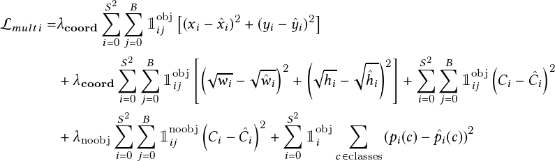 | (2.2) |
where 1iobj denotes if the object appears in cell i and 1ijobj denotes that the jth bounding box predictor in cell i is “responsible” for that prediction. The remaining variables are as follows: �coord and �noobj are the bounding box coordinate predictions and the confidence score predictions for boxes without objects. S is the number of cells an image is split along an axis, resulting in S �S cells. B is the number of bounding box locations predicted by each cell. A tuple of four values defines the coordinates of the bounding box (x,y,w,h) where x and y are the centers of the bounding boxes xi (yi, wi, hi), and xi (ŷi, ŵi, ĥi) are the ground truth and prediction, respectively, of x (y, w, h). Ci is the confidence score of cell i, whereas Ĉi is the predicted confidence score. Finally, Pi is the conditional probability of cell i containing an object of a class, whereas Pi is the predicted conditional class probability.
MOT can generally be regarded as a multivariable estimation problem [53]. The objective of MOT can be modeled by performing MAP (maximum a posteriori) estimation to find the optimal sequential states of all the objects from the conditional distribution of the sequential states, given all the observations:
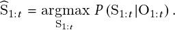 | (2.3) |
where St = �st1;st2;:::;stMt� denotes states of all the Mt objects in the t-th frame, and sti denotes the state of the i-th object in the t-th frame. S1:t = fS1;S2;…;Stg denotes all the sequential states of all the objects from the first frame to the t-th frame. In tracking-by-detection, oti denotes the collected observations for the i-th object in the t-th frame. Ot = �ot1;ot2;…;otMt� denotes the collected observations for all the Mt objects in the t-th frame. O1:t = fO1;O2;…;Otg denotes all the collected sequential observations of all the objects from the first frame to the t-th frame.
Due to single-frame inputs, the spatial stream network cannot extract motion features and compute trajectories. To leverage this helpful information, we present our temporal stream network. This ConvNet model implements a tracking-by-detection MOT algorithm [49, 52] with a data association metric that combines deep appearance features. The inputs are identical to the spatial stream network using the original video. Detected object candidates (only vehicle classes) are used for tracking, state estimation, and frame-by-frame data association using SORT [49] and DeepSORT [52]—the real-time MOT method. MOT models each object’s state and describes objects’ motion across video frames. The tracking information allows us to stack trajectories of moving objects across several consecutive frames, which are useful cues for near-accident detection.
Estimation Model For each target, its state is modeled as
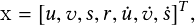 | (2.4) |
where u;v denotes the 2D pixel location of the target’s center. The variable s denotes the scale of the target’s bounding box, and r is the aspect ratio (usually considered constant). The target’s state is updated when a newly detected bounding box is associated with it by solving the velocity via a Kalman filter [50]. The target’s state is predicted (without correction via the Kalman filter if no bounding box is associated.
Data Association To assign all new detection boxes to existing targets, we predict each target’s new location (one predicted box) in the current frame and compare the IoU distance between new detection boxes and all predicted boxes (the detection-to-target overlaps), forming the assignment cost matrix. The matrix is further used in the Hungarian algorithm [51] to solve the assignment problem. One assignment is rejected if the detection-to-target overlap is less than a threshold (the minimum IoU, IoUmin). The IoU distances of the bounding boxes are utilized to handle the short-term occlusion caused by passing targets.
Creation and Deletion of Track Identities. When new objects enter or old objects vanish in video frames, we must add or remove certain tracks (or objects) to maintain unique identities. We treat any detection that fails to associate with existing targets as one potential untracked object. This target undergoes a probationary period to accumulate enough evidence by associating the target with detection. This strategy can prevent the tracking of false positives. The track object is removed from the tracking list if it remains undetected for TLost frames, which enables maintenance of a relatively unbounded number of trackers and reduces localization errors accumulated over a long duration.
Track Handling and State Estimation. This part is mostly identical to SORT [49]. The tracking scenario is represented as an eight-dimensional state space �u;v;�;h;ẋ;ẏ;�;ḣ�. The pair �u;v� represents the bounding box center location. � is the aspect ratio, and h is the height. The rest are the bounding box’s velocities relative to other bounding boxes. This representation is used to describe the constant velocity motion, (ẋ;ẏ;�;ḣ�, and linear observation model, (u;v;�;h), in Kalman filtering [50].
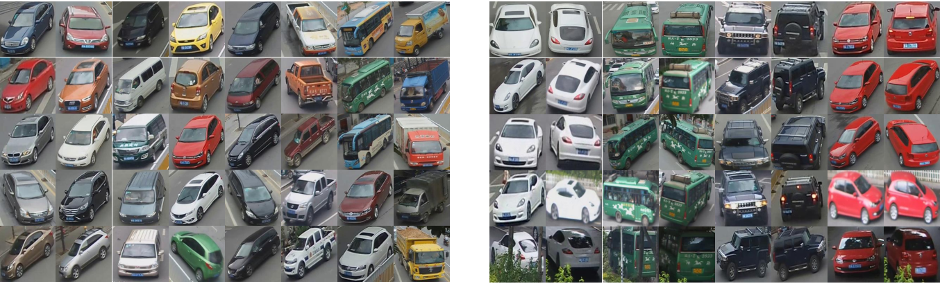
| Figure 2.5.: | Vehicle samples selected from the VeRi dataset [54]. All images are the same size, and we resize them to 64 � 128 for training. Left: Diversity of vehicle colors and types; right: variation of the viewpoints, illuminations, resolutions, and occlusions for the vehicles. |
Data Association To solve the frame-by-frame association problem, SORT uses the Hungarian algorithm [51], where both motion and appearance information is considered.
The (squared) Mahalanobis distance is utilized to measure the distance between newly arrived measurements and Kalman states:
 | (2.5) |
where yi and dj denote the i-th track distribution and the j-th bounding box detection, respectively. The smallest cosine distance between the i-th track and j-th detection is considered to handle appearance information:
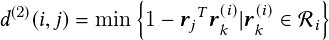 | (2.6) |
where both motion and appearance are combined linearly, and a hyperparameter, �, controls the influence of each:
 | (2.7) |
Matching Cascade. Previous methods tried to solve measurement-to-track associations globally, while SORT adopts a matching cascade introduced in [52] to solve a series of subproblems. In some situations, when an object is occluded for a more extended period, the subsequent Kalman filter [50] predictions would increase the uncertainty associated with the object location. Consequently, the probability mass will spread out in the state space and the observation likelihood will decrease. The measurement-to-track distance should be increased by considering the spread of probability mass. Therefore, objects seen more frequently are prioritized in the matching cascade strategy to encode the notion of probability spread in the association likelihood.
Metric learning and various hand-crafted features are widely used in person re-identification problems. We apply a cosine metric learning method to train a neural network for vehicle re-identification and use it to make our temporal stream more robust regarding tracking performance. Metric learning aims to solve the clustering problem by constructing an embedding in which the metric distance corresponding to the same identity is likely closer than features from different identities. The cosine metric measures the degree of similarity by calculating the cosine distance between two objects. We observe that our tracking algorithm produces switched road user identities in traffic video, especially in crowded traffic scenes or scenes with heavy occlusion. In order to generate accurate and consistent track data, we introduce a deep cosine metric learning method to learn the cosine distance between objects. The cosine distance involves appearance information that provides valuable cues for recovering identities in crowded scenes or after long-term occlusion when motion information is less discriminative. Through this deep network, the feature expression vector obtained by any object is placed in the cluster corresponding to the nearest neighbor. We trained the network on a vehicle re-identification dataset (VeRi dataset) [54] (Figure 2.5) and integrated it as the second metric measure for the assignment problem of our temporal stream.
We aim to use a unified end-to-end framework that automatically learns the best metrics. Compared to the standard distance metric (L1, L2), the learned metric can obtain more discriminative features for re-identification and is more robust to cross-view vehicle images. We adopt the architecture of [55] and train a deep network with a cosine softmax classifier that can generate feature vectors of fixed length (128) for the input images (vehicles). The cosine metric finds the nearest cluster exemplar and matches the vehicle on (sometimes far-flung) different video frames to solve tracking problems in heavy occlusion.
Given a re-identification dataset D = f�xi;yi�gi=1N of N training images xi 2 RD and associated class labels yi 2 f1;…;Cg, deep metric learning is used to find a parameterized encoder function. The deep metric neural network is r = f�� input� with parameters �, which projects the input images x 2 RD into a feature representation, r 2 Rd, that follows a predefined notion of cosine similarity.
The cosine softmax classifier can be adapted from a standard softmax classifier and is expressed as
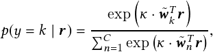 | (2.8) |
where � is a free scale parameter. To generate compact clusters in the feature representation space, the first modification is to apply the `2 normalization to the final layer of the encoder network so that the representation has unit length kf��x�k2 = 1;[x 2 RD. The second modification is to normalize the weights to unit length as well, i.e., wk = wk�kwkk2;[k = 1;…;C. The training of the encoder network can be carried out using the cross-entropy loss as usual. In particular, the authors in [56] have proposed accelerating the convergence of stochastic gradient descent by decoupling the length of the weight vector � from its direction.
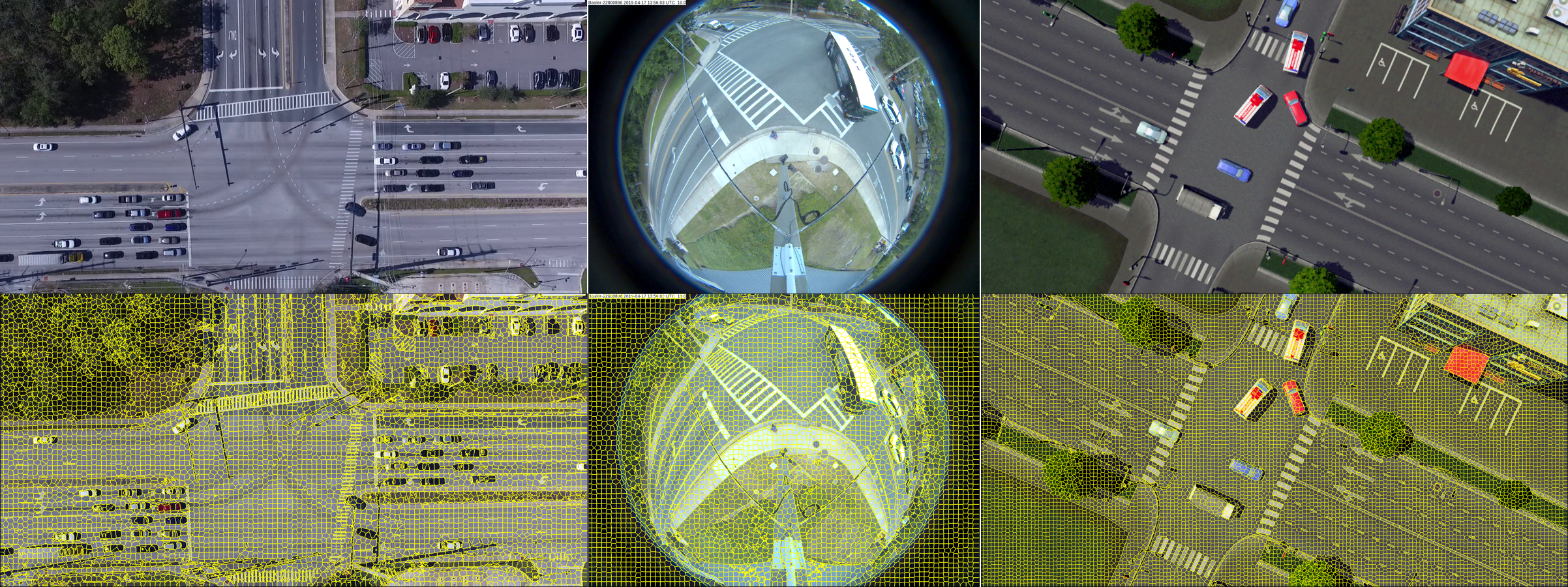
| Figure 2.6.: | 2D image superpixel segmentation using SLIC [57]. Top: original image; bottom-left: SLIC segmentation for drone video (1,600 superpixels); bottom-middle: SLIC segmentation for fisheye video (1,600 superpixels); bottom-right: SLIC segmentation for simulation video (1,600 superpixels). |
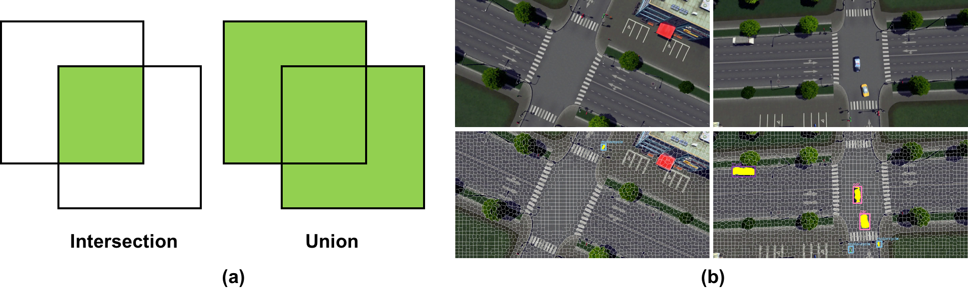
| Figure 2.7.: | An illustration depicting the segmentation mask. (a) An illustration depicting the definitions of intersection and union. (b) Top: original video frames; bottom: object detections and object masks produced by our method. |
To present our method fully end-to-end, we apply a learning-based dynamic distance threshold rather than a manually defined one to determine near-accident detection. A near-accident is detected if the distance between two objects in the image space is below the threshold. Using object segmentation, we introduce a threshold-learning method by estimating the gap between objects. We present a supervised learning method, using the gap distance between road users in the temporal stream to determine a near-accident while continuing to update the threshold for more convergence and precision. The straightforward way is to compute the gap using bounding boxes from detections. Still, the bounding boxes need to be more accurate in representing the boundaries of objects, particularly when rotation is involved. Therefore, we need a more compact representation and combine detections with superpixel segmentation on the video frame to get an object mask for gap distance estimation.
The main steps of our gap estimation method can be summarized as follows:
In our gap estimation methods, the Intersection over Union (IoU) metric of boxes and superpixels is given by
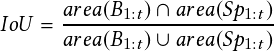 | (2.9) |
where Bt = �bt1;bt2;:::;btMt� denotes the collected detection observations for all the Mt objects in the t-th frame, and bti denotes the detection for the i-th object in the t-th frame. B1:t = fB1;B2;:::;Btg denotes all the collected sequential detection observations of all the objects from the first frame to the t-th frame. Similarly, Spt = �spt1;spt2;:::;sptNt� denotes all the Nt superpixels in the t-th frame, and spti denotes the i-th superpixel in the t-th frame. Sp1:t = fSp1;Sp2;:::;Sptg denotes all the collected sequential superpixels from the first frame to the t-th frame.
In 2D superpixel segmentation, the popular SLIC (simple linear iterative clustering) [57] and ultrametric contour map (UCM) [58] methods have established themselves as the state-of-the-art. Recently, we have seen deep neural networks [59] and generative adversarial networks (GANs) [60] integrated with these methods. In our architecture, we adopt the GPU-based SLIC (gSLICr) [22] approach to produce the tessellation of the image data to achieve an excellent frame rate (400 fps). SLIC is widely applicable to many computer vision applications, such as segmentation, classification, and object recognition, often achieving state-of-the-art performance. The contours forming the homogeneous superpixels are shown in Figure 2.6. In Figure 2.7, we illustrate the definition of intersection and union and present some object masks we generated from detections and superpixels.
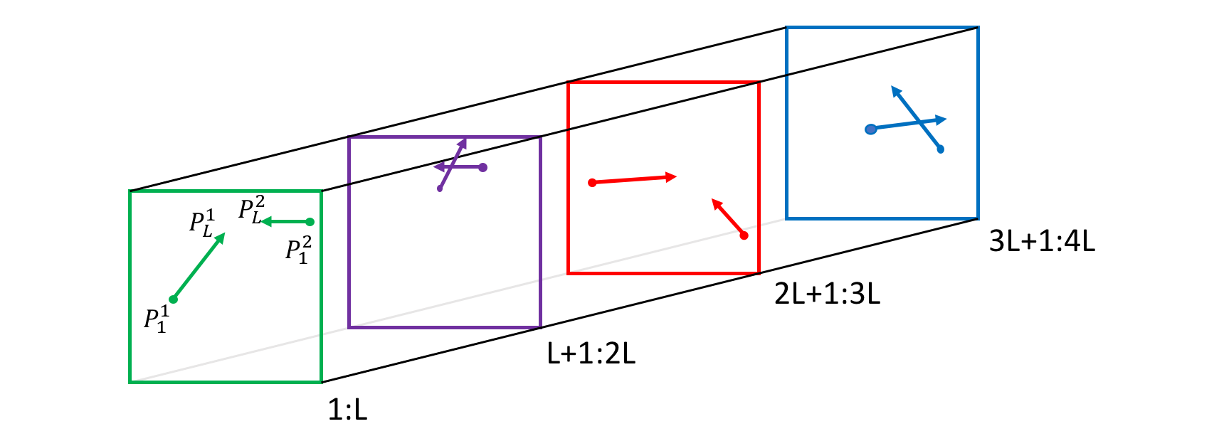
| Figure 2.8.: | The stacking trajectories extracted from multiple object tracking of the temporal stream. Consecutive frames and the corresponding displacement vectors are shown with the same color. |
The most typical motion cue is optical flow, which is widely utilized in video processing tasks such as video segmentation [61]. A trajectory is a data sequence containing several concatenated state vectors from tracking and an indexed sequence of positions and velocities over a given time window.
When utilizing the multiple object tracking algorithm, we compute the center of each object in several consecutive frames to form stacking trajectories as our motion representation. These stacking trajectories can provide accumulated information through image frames, including the number of objects, their motion history, and the timing of their interactions, such as near-accidents. We stack the trajectories of all objects for L consecutive frames, as illustrated in Figure 2.8, where pti denotes the center position of the i-th object in the t-th frame. Pt = �pt1;pt2;…;ptMt� denotes trajectories of all the Mt objects in the t-th frame. P1:t = fP1;P2;…;Ptg denotes the sequence of trajectories of all the objects from the first frame to the t-th frame. For L consecutive frames, the stacking trajectories are defined by the sequence
 | (2.10) |
Ot = �ot1;ot2;…;otMt� denotes the collected observations for all the Mt objects in the t-th frame. O1:t = fO1;O2;…;Otg denotes all the collected sequential observations of all the objects from the first frame to the t-th frame. We use a simple detection algorithm that finds collisions between simplified forms of the objects using the center of bounding boxes.
Our algorithm is depicted in Algorithm 1. Once a collision is detected, we set the region covering collision-associated objects as a new bounding box with a class probability of near-accident as 1. We can obtain a final confidence measure of near-accident detection by averaging the near-accident probabilities from the spatial stream network and the temporal stream network.
Here, we present qualitative and quantitative evaluations regarding object detection, MOT, and near-accident detection performance. We also compare other methods with our framework.
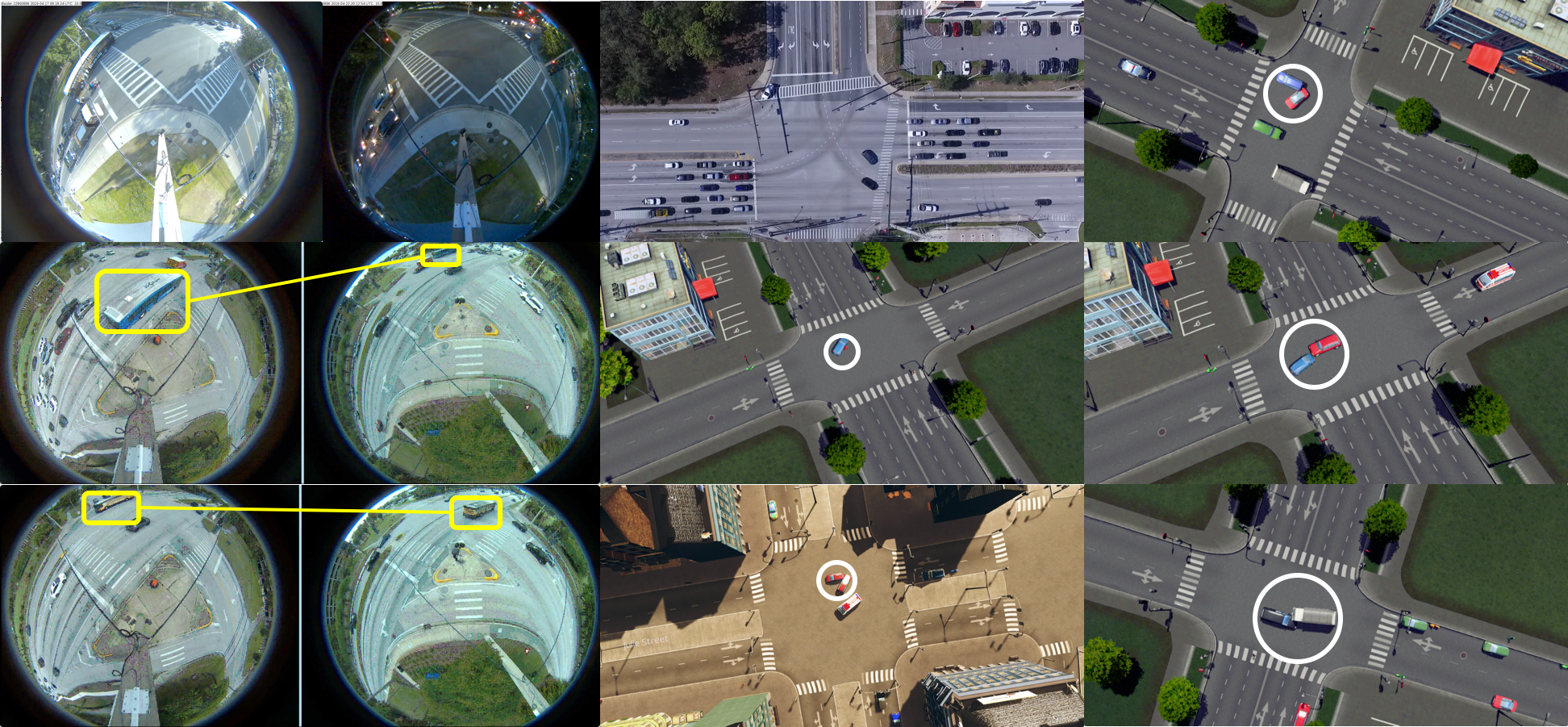
| Figure 2.9.: | Samples of traffic near-accident: Our data consists of many diverse intersection surveillance videos and near-accidents (cars and motorbikes). Yellow rectangles and lines represent the same object in video from multiple cameras. White circles represent the near-accident regions. |
To our best knowledge, we know of no comprehensive traffic near-accident dataset containing top-down-view videos such as drone or UAV videos or omnidirectional camera videos for traffic analysis. Therefore, we have built our traffic near-accident dataset (TNAD), depicted in Figure 2.9. Intersections tend to experience more near-accidents and more potentially severe ones due to factors such as angles and turning collisions. The traffic near-accident dataset contains three types of video data from traffic intersections that could be utilized for near-accident detection and other traffic surveillance tasks, including turn movement counting.
The first type is drone video that monitors an intersection with a top-down view. The second type of intersection video is real traffic video acquired by omnidirectional fisheye cameras that monitor small or large intersections. They are widely used in transportation surveillance. These video data can be directly used as input for our vision-based intelligent framework. Furthermore, preprocessing and fisheye correction can be applied for better surveillance performance. The third type of video is video game-engine simulations that train on near-accident samples as they are accumulated. The dataset consists of 106 videos with a total duration of over 75 minutes, with frame rates between 20 and 50 fps. The drone and fisheye surveillance videos were recorded in Gainesville, Florida, at several intersections. Our videos are more challenging than videos in other datasets for the following reasons:
We manually annotated the spatial and temporal locations of near-accidents, the still or moving objects, and their vehicle class in each video. Thirty-two videos with sparsely sampled frames (only 20% of the frames in these 32 videos are used for supervision) were used, but only for training the object detector. The remaining 74 videos were used for testing.
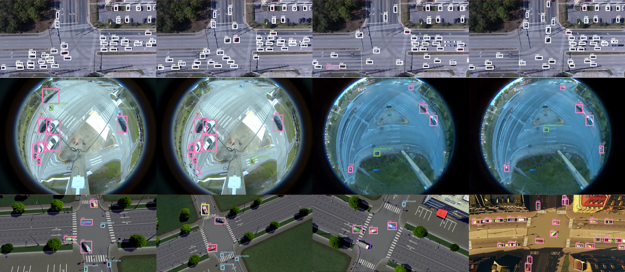
| Figure 2.10.: | object detection result samples of our spatial network on TNAD dataset. Top: samples for drone video; middle: samples for fisheye video; bottom: samples for simulation video. |
We have large amounts of fisheye traffic videos from across the city. The fisheye surveillance videos were recorded from real traffic data in Gainesville. We collected 29 single-camera fisheye surveillance videos and 19 multi-camera fisheye surveillance videos monitoring a large intersection. We conducted two experiments, one directly using these raw videos as input for our system and another in which we first preprocessed the video to correct fisheye distortion and then fed them into our system. As the original surveillance video has many visual distortions, especially near the circular boundaries of the cameras, our system performed better on these after preprocessing. In this chapter, we do not discuss issues related to fisheye unwarping, leaving these for future work.
For large intersections, two fisheye cameras placed opposite each other are used for surveillance, showing almost half the roads and real traffic. We apply a simple object-level stitching method by assigning the object identifier for the same objects across the left and right videos using similar features and appearing and vanishing positions.
We adopt Darknet-19 [52] for classification and detection with DeepSORT, using a data association metric that combines deep appearance features. We implement our framework on Tensorflow and perform multiscale training and testing with a single GPU (NVIDIA Titan X Pascal). Training a single spatial convolutional network takes one day on our system with one NVIDIA Titan X Pascal card. We use the same training strategy for classification and detection training as YOLO9000 [52]. We train the network on our dataset with four classes of vehicle (motorbike, bus, car, and truck) for 160 epochs, using stochastic gradient descent with a starting learning rate of 0.1 for classification and 10�3 for detection (dividing it by ten at 60 and 90 epochs.), weight decay of 0.0005, and momentum of 0.9 using the darknet neural network framework [52].
![]()
| Figure 2.11.: | Tracking and trajectory comparison with Urban Tracker [62] and TrafficIntelligence [63] on drone videos of TNAD dataset. Left: tracking results of Urban Tracker [62] (BSG with Multilayer and Lobster Model; middle: tracking results of TrafficIntelligence [63]; right: tracking results of our temporal stream network. |
We present some example experimental results of object detection MOT, and near-accident detection on our traffic near-accident dataset (TNAD) for drones, fisheye, and simulation videos. For object detection (Figure 2.10), we present some detection results of our spatial network with multiscale training based on YOLOv2 [47]. These visual results demonstrate that the spatial stream is able to detect and classify road users with reasonable accuracy, even if the original fisheye videos have significant distortions and occlusions. Unlike drone and simulation videos, we have added pedestrian detection on real traffic fisheye videos. From Figure 2.10, our detector performs well on pedestrian detection for daylight and dawn fisheye videos. The vehicle detection capabilities are good on top-down view surveillance videos, even for small objects. In addition, we can achieve a fast detection rate of 20 to 30 frames per second. Overall, this demonstrates the effectiveness of our spatial neural network.
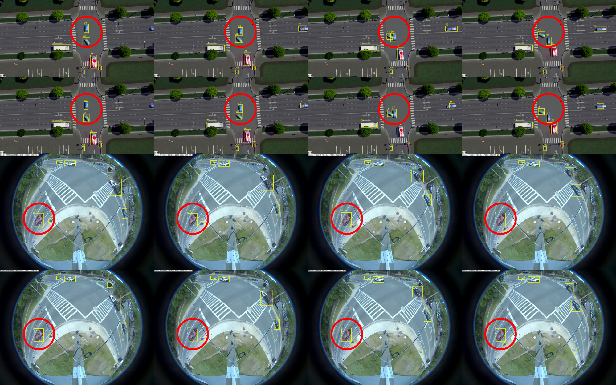
| Figure 2.12.: | Multiple Object Tracking (MOT) comparisons of our baseline temporal stream (SORT) with cosine metric learning-based temporal stream. Row 1: results from SORT (ID switching issue); row 2: results from cosine metric learning + SORT (ID consistency); row 3: results from SORT (ID switching issue); row 4: results from cosine metric learning + SORT (ID consistency). |
For MOT (Figure 2.11), we present a comparison of our temporal network based on DeepSORT [52] with Urban Tracker [62] and TrafficIntelligence [63]. We also present more visual MOT comparisons of our baseline temporal stream (DeepSORT) with cosine metric learning-based temporal stream (Figure 2.12). For the tracking part, we use a tracking-by-detection paradigm; thus, our methods can handle still objects and measure their state. This is especially useful because Urban Tracker [62] and TrafficIntelligence [63] can only track moving objects. On the other hand, Urban Tracker [62] and TrafficIntelligence [63] can compute dense trajectories of moving objects with reasonable accuracy, but they have slower tracking speed—around one frame per second. Our two-stream convolutional networks can do spatial and temporal localization for accident detection for diverse accident regions involving cars and motorbikes. The three subtasks (object detection MOT, and near-accident detection) can consistently achieve real-time performance at a high frame rate—40 to 50 frames per second—and this depends on the frame resolution (e.g., 50 fps for 960�480 image frames).
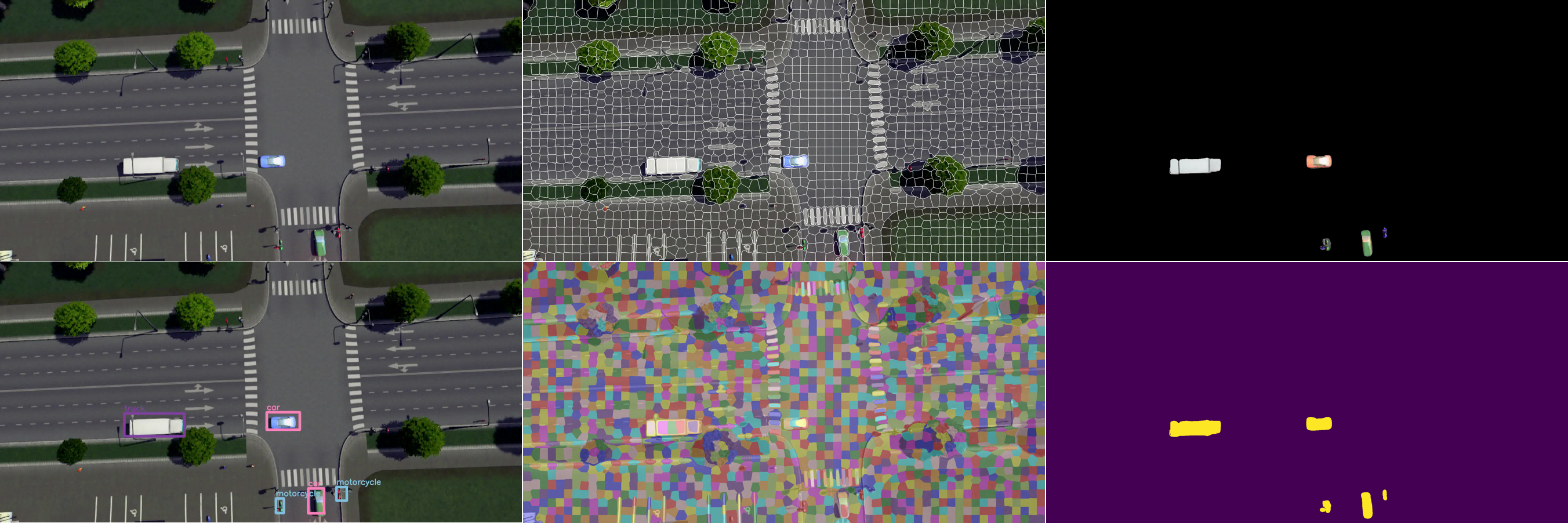
| Figure 2.13.: | Object segmentation using detections and superpixels. Top-left: original image; top-middle: superpixels generated by SLIC [57]; top-right: final object mask; bottom-left: object detections; bottom-middle: colored superpixels generated by SLIC [57]; bottom right: final binary object mask. |
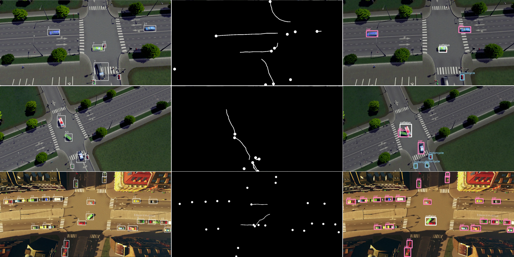
| Figure 2.14.: | Sample results of tracking, trajectory, and near-accident detection of our two-stream convolutional networks on simulation videos of TNAD dataset. Left: tracking results from the temporal stream; middle: trajectory results from the temporal stream; right: final near-accident detection results from the two-stream convolutional networks. |
In Figure 2.12, we demonstrate the effectiveness of applying cosine metric learning with the temporal stream for solving ID switching (and for the case where new object IDs emerge). For example, the first row shows that the ID of the green car (inside the red circle) got changed from 32 to 41. The third row shows that the IDs of the red car and a pedestrian (inside the red circle) were changed (from 30 to 43 and 38 to 44, respectively). The second and fourth rows demonstrate that with cosine metric learning, the IDs of tracks are kept consistent. In Figure 2.13, we show an example of a more accurate and compact road user mask generated by superpixel segmentation and detections for the learning-based gap estimation. With a segmentation mask, we can estimate the gap distance between road users more accurately than directly using object detections. Segmentation would be more beneficial for fisheye videos where the distortion is significant, and occlusion is heavier. For near-accident detection (Figure 2.14), we present final near-accident detection results along with tracking and trajectories using our two-stream convolutional networks method. Overall, the qualitative results demonstrate the effectiveness of our spatial and temporal networks.
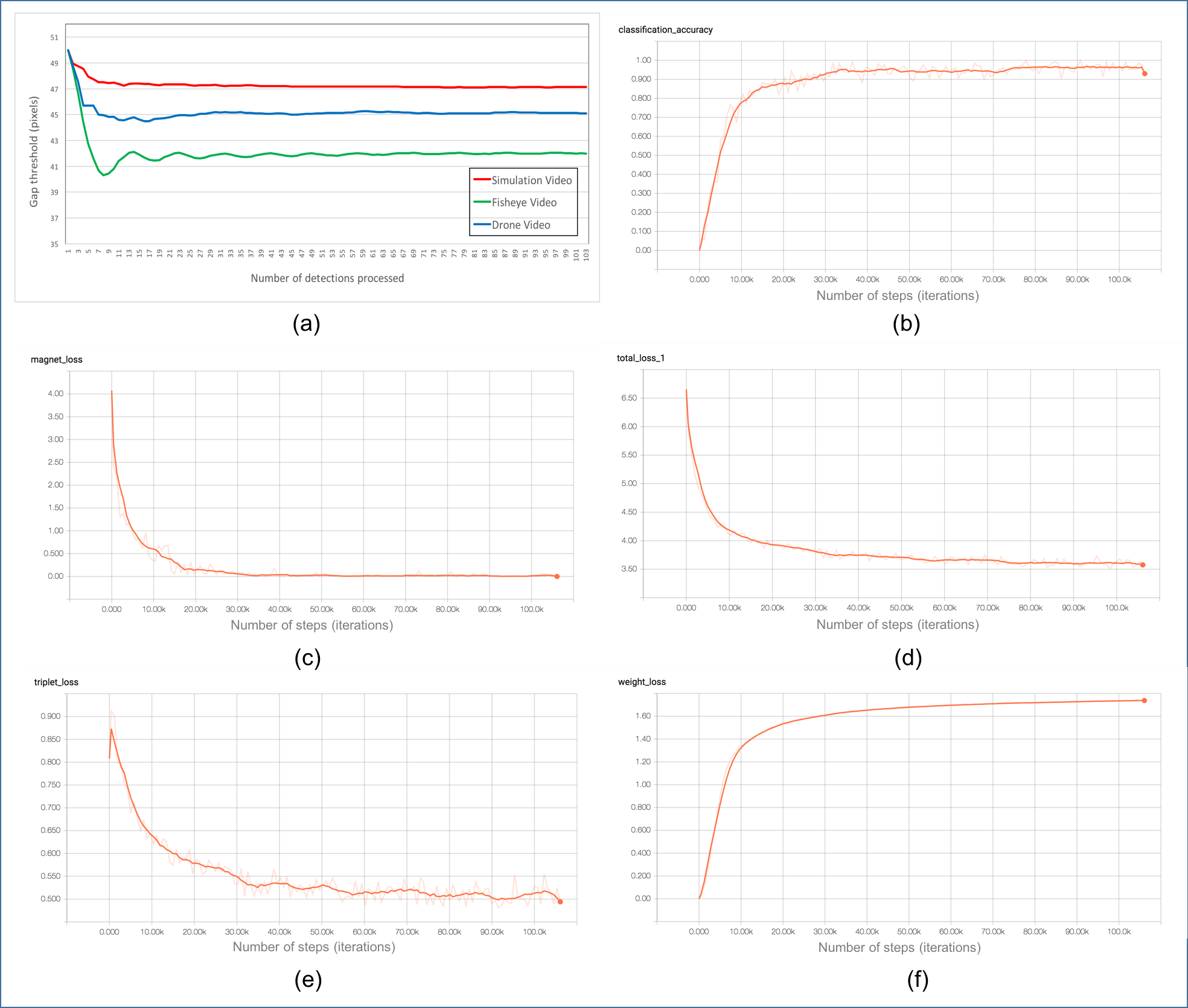
| Figure 2.15.: | Gap estimation and cosine metric learning. (a) Evolution of gap threshold for three types of videos; (b) classification accuracy for training VeRi dataset; (c) evolution of total loss for training; (d) evolution of magnet loss for training; (e) evolution of triplet loss for training; (f) evolution of weight loss for training. |
We present timing results for the tested methods in Table 2.1. All experiments have been performed on a single GPU (NVIDIA Titan V). The GPU-based SLIC segmentation [57] has excellent speed and runs from 110 to 400 fps on videos of different resolutions. The two-stream CNNs (object detection, MOT, and near-accident detection) can achieve real-time performance at a high frame rate, 33–50 fps, depending on the frame resolution.
We present some quantitative results for gap estimation and cosine metric learning in Figure 2.15. The results for cosine metric learning have been established after training the network for a fixed number of steps (100,000 iterations). The batch size was set to 120 images, and the learning rate was 0:001. All configurations after training have fully converged, as depicted in Figure 2.15.
| Table 2.1.: | Quantitative evaluation of timing results for the tested methods. |
|
Methods |
GPU | Drone | Simulation | Fisheye | |
| 1920 � 960 | 2560 � 1280 | 3360 � 1680 | 1280 � 960 | ||
| SLIC segmentation | Nvidia Titan V | 300 fps | 178 fps | 110 fps | 400 fps |
| Two-Stream CNNs | Nvidia Titian V | 43 fps | 38 fps | 33 fps | 50 fps |
| Table 2.2.: | Quantitative evaluation of all tasks for our two-stream method. |
| Task or Methods | Data | Precision | recall | F1-score | |
|
object detection | Simulation | 0.92670 | 0.95255 | 0.93945 | |
| Fisheye | 0.93871 | 0.87978 | 0.90829 | ||
|
multiple object tracking | Simulation | 0.89788 | 0.86617 | 0.88174 | |
| Fisheye | 0.91239 | 0.84900 | 0.87956 | ||
| Simulation | 0.91913 | 0.90310 | 0.91105 | |
| Fisheye | 0.92663 | 0.87725 | 0.90127 | ||
| SLIC Segmentation Mask | Simulation | 0.93089 | 0.81321 | 0.86808 | |
| Simulation | 0.90395 | 0.86022 | 0.88154 | |
| Simulation | 0.83495 | 0.92473 | 0.84108 | |
| Simulation | 0.92105 | 0.94086 | 0.93085 | |
Triplet Loss. The triplet loss for cosine metric learning network [64] is defined by
 | (2.11) |
where ra, rp, and rn are three samples in which a positive pair, ya = yp, and a negative pair, ya < yn, are included. With a predefined margin m 2 R, the triplet loss demands the distance between the positive and negative is larger than it. In this experiment, we introduce a soft-margin–based triplet loss where we replace the hinge of the original triplet loss [65] by a soft plus function,  � = log�1 � exp�x��, to resolve non-smoothness [66] issues. Further, to avoid potential issues
in the sampling strategy, we directly generate the triplets on GPU as proposed by [65].
� = log�1 � exp�x��, to resolve non-smoothness [66] issues. Further, to avoid potential issues
in the sampling strategy, we directly generate the triplets on GPU as proposed by [65].
Magnet Loss. Magnet loss is defined as a likelihood ratio measure that demands the separation of all samples away from the means of other classes. Instead of using a multimodal form in its original proposition [66], we use a unimodal, adapted version of this loss to fit the vehicle re-identification problem:
 | (2.12) |
where �y�= f1;…;Cgnfyg, and the m is the predefined margin parameter, �y is used to represent the sample mean of class y, and �2 denotes the variance of each sample separated away from their class mean. They are all established for each batch individually on GPU.
For learning the gap threshold with superpixel segmentation and detections, the plot (Figure 2.15, top left) demonstrates the converging evolution of gap distance for three types of video. The initial gap threshold is set to be 50 pixels; the average gap thresholds from experiments are about 47 pixels, 45 pixels, and 42 pixels for simulation video, fisheye video and drone video, respectively.
The evaluation method we use, for instance segmentation, is quite similar to object detection, except that we now calculate the IoU of masks instead of bounding boxes.
Mask Precision, recall, and F1 Score. To evaluate our collection of predicted masks, we’ll compare each of our predicted masks with each of the available target masks for a given input.
Since our framework has three tasks and our dataset is quite different from other object detection datasets, tracking datasets, and near-accident datasets such as dashcam accident dataset [67], it isn’t easy to compare the individual quantitative performance for all three tasks with other methods. One of our motivations was to propose a vision-based solution for ITS; therefore, we focus more on near-accident detection and present a quantitative analysis of our two-stream convolutional networks. In Table 2.2, we present quantitative evaluations of three subtasks: object detection; multiple object tracking (with and without cosine metric learning); SLIC segmentation (mask vs. bounding box); and near-accident detection (spatial stream only, temporal stream only, and two-stream model). We present evaluations regarding object detection and multiple objects tracking for the fisheye video. The simulation videos are for training and testing with more near-accident samples, and we have 57 simulation videos totaling over 51,123 video frames. We sparsely sample only 1,087 frames from them for training processing. We present the analysis of near-accident detection for 30 testing videos (18 had positive near-accident; 12 had negative near-accident).
Near-accident Detection Precision, recall, and F1 Score. We’ll compare our predicted detections with each ground truth for a given input to evaluate our prediction of near-accidents.
We have proposed a two-stream convolutional network architecture that performs real-time detection, tracking, and near-accident detection for vehicles in traffic video data. The two-stream convolutional network comprises a spatial and temporal stream network. The spatial stream network detects individual vehicles and likely near-accident regions at the single-frame level by capturing appearance features with a state-of-the-art object detection method. The temporal stream network leverages motion features of detected candidates to perform multiple object tracking and generates individual trajectories of each tracked target. We detect near-accidents by incorporating appearance and motion features to compute probabilities of near-accident candidate regions. Experiments have demonstrated the advantage of our framework with an overall competitive qualitative and quantitative performance at high frame rates. Future work will include image stitching methods deployed on multi-camera fisheye videos.
We develop a novel workflow for analyzing vehicular and pedestrian traffic at an intersection, beginning with ingesting video data and controller logs, followed by data storage and processing to generate dominant and anomalous behavior at the intersection, which helps in various applications such as near-miss detection [68], which is explained in detail in this chapter. The critical contributions of the work in this chapter are as follows:
Extensive results are provided on video and signal data collected at an intersection. These results demonstrate that video and signal timing information is useful in quantifying
The rest of the chapter is organized as follows. Section 3.2 describes the trajectory generation in brief, and Section 3.3 describes the recording of the current signal state of an intersection. Finally, Section 3.4 presents a detailed comparison of the candidate distance measures. Sections 3.7-3.9 presents an exhaustive treatise on near-miss detection.
Video processing software processes object locations frame by frame from a video and outputs the location coordinates along with the corresponding timestamp. The video is captured by a camera installed at an intersection. To accurately locate the coordinates of an object, the video processing software must account for the different types of distortions that creep into the system. For example, a fisheye lens would have significant radial distortion. After taking into account the intrinsic and extrinsic properties of the camera, a mapping is created, which is used by the video processing software to map observed coordinates to modified coordinates that are nearly free of any distortion. To represent the location of a 3D object using a dimensionless point, one looks to find the object’s center of mass. A bounding box is drawn, enclosing the object. The center of the box is approximated to be the object’s center of mass. After generating timestamped trajectory coordinates, the software computes other properties, such as speed and direction of movement.
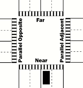
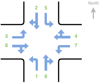
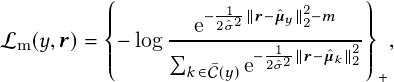
An intersection almost always has traffic lights to control traffic flow safely. The signal changes from green to yellow to red are events captured in controller logs called signal data. To specify a particular signal and, in a more general sense, the direction of movement, the traffic engineers define a standard that assigns phases 2 and 6 to the two opposite directions of the major street and 4 and 8 to those of the minor street. Figure 3.1 shows these phase numbers and the phase numbers for the turning vehicles and pedestrians.
Our application stores the current signal phase in a compact 6-digit hexadecimal encoding. To explain the formatting, let us consider the corresponding 24-bit binary equivalent. The bits 1–8 are programmed to be 1 if the corresponding phase is green and 0 otherwise. Similarly, bits 9–16 and 17–24 are reserved for programming the yellow and red status for the eight-vehicle phases, respectively. For example, green on phases 2 and 6 at an intersection would have a binary encoding of 0100 0100 for the first 8 bits, the next eight bits would be 0000 0000 for yellow, and the last set of 8 bits for red would be one where the second and sixth bits are 0 represented as 1011 1011. Thus, the overall 24-bit binary representation of the current signaling state is 0100 0100 0000 0000 1011 1011, or 4400bb.
| Figure 3.1.: | Phase Diagram showing vehicular and pedestrian movement at four-way intersections. The solid gray arrows show vehicle movements while the blue dotted arrows show pedestrian movements [69]. |
The first step toward clustering a set of trajectories is applying a suitable distance measure that will, for any two trajectories, tell how close the trajectories are to each other in space and time. Two potential candidates for distance measures of the intersection trajectories are euclidean distance (ED) and dynamic time warping (DTW). Among these, ED is the square root of the sum of the squared length of vertical or horizontal hatched lines. The disadvantage of using ED is that it cannot calculate their distance reliably for trajectories of different sizes.
DTW can compute distances between trajectories when they vary in time, speed, or path length. Although DTW utilizes a dynamic programming approach for an optimal distance and has time complexity O�N2�, where N is the number of coordinates in the two trajectories, there are approximate approaches such as FastDTW that realize a near-optimal solution and has a space and time complexity of O�N�. FastDTW is based on a multilevel iterative approach. FastDTW returns a distance and a list of pairs of points, also known as the warp path. A pair of points consists of coordinates on the first and second trajectories and represents the best match between the points after the trajectories are warped. The distance returned by FastDTW is the sum of the distances between each pair of points on the path. Quite naturally, the distance is negligible if the trajectories occur in the same geographical coordinates and are traversed at similar speeds.

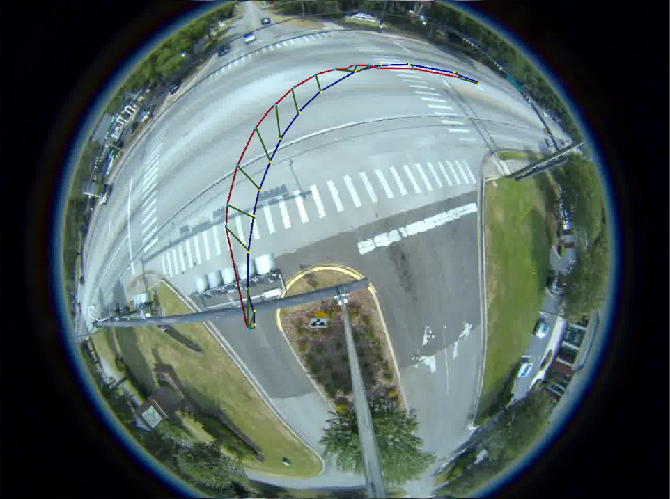
| Figure 3.3.: | An example where two similar trajectories have a high distance value when DTW/FastDTW is directly used to compute distance. This is potentially due to differential tracking of vehicles due to potential occlusion. |
DTW and FastDTW work well for trajectories entirely captured by the sensor system. In reality, the sensor system and the processing software may not wholly capture the trajectory. In that case, the distance the dynamic time-warping algorithm returns does not represent the actual distance. Figure 3.3 highlights two example trajectories for which DTW returns a high value for the distance suggesting the tracks are dissimilar. For example, for the two tracks
going straight, if the starting portion of one of the tracks is truncated due to a processing error, as shown in Figure 3.4, the distance between the tracks will be  . Thus, the distance computed results in a high value, which often falls in the distance range between two unrelated trajectories. Hence, we developed a new distance measure by utilizing the warp path returned by the
FastDTW.
. Thus, the distance computed results in a high value, which often falls in the distance range between two unrelated trajectories. Hence, we developed a new distance measure by utilizing the warp path returned by the
FastDTW.
We describe our trajectory clustering method in this section. There are two main components to clustering; the first is to use an efficient distance measure for the trajectories to be clustered, and the second is to use a clustering algorithm that uses the distance measure to create clusters of trajectories that behave similarly. We describe the novel distance measure developed as part of this work in Section 3.5.1 and present our clustering algorithm in Section 3.5.2.
The new distance measure developed in this section applies to trajectories captured using real-time video processing.
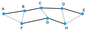
| Figure 3.4.: | Two trajectories represented by ABCDE and FGH. The dashed lines show the point correspondence (warp path) obtained using FastDTW. The trajectory FGH is shorter because the beginning part of the trajectory was not captured. |
The first step in the computation of the distance measure is to obtain the warp path using a time-warping algorithm, e.g., FastDTW. Triangles are constructed using the warp path as shown in Figure 3.4, where the triangles are 4ABF, 4BCF, 4CDF, 4DFG, 4DEG, and 4EGH. Since the coordinates of the vertices (A, B, C, D, E, F, G, and H) are known, the area of each may be computed using the following formula from coordinate geometry.
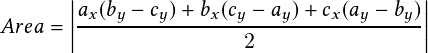 | (3.1) |
where the vertices of the triangle have coordinates: �ax;ay�;�bx;by�; and �cx;cy�. The sum of the area of all triangles is computed, and finally, the distance, Dij, between two trajectories Ti and Tj, is computed as:
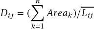 | (3.2) |
where Areak is the area of the kth triangle and Lij is the average length of the two trajectories, Ti and Tj, and n is the total number of triangles. If there is no warping, and the number of matched pairs is m, then n = 2m, by construction. However, if there is warping, then n < 2m. Dij is the average perpendicular distance between the trajectories, which intuitively is the average height of the triangles.
To get a more accurate local distance measure, we segment the trajectories and compute the distance of the starting and the finishing segments. Let SDij and FDij be the distances of the starting and the finishing segments, respectively. Then, SDij is the distance between the first pair of matching points that are not warped (CF and DG in Figure 3.4), and correspondingly, FDij is the distance between the last pair of matching points that are not warped (DG and EF in Figure 3.4). SDij may be computed as the average height of triangles 4CFG and 4CDG, and FDij as that of triangles 4DGH and 4DEH. Thus, we use triplets of (Dij, SDij, FDij) to represent the distance between two trajectories. If required, these three portions of the distance measure can be suitably weighted for computing a scalar distance.
The similarity matrix, S, is computed from the distance measures by setting up empirical thresholds for the magnitude of the distance between two trajectories. For example, given two trajectories Ti and Tj, if their average distance, Dij, from Equation 3.2 is less than a threshold �x and the start section distance, SDij, is less than a threshold �y and the last section distance, FDij, is less than a threshold �z, then Ti and Tj are considered similar. In that case, the corresponding entry in the similarity matrix would be Sij = Sji = 1. If any distance value exceeds the corresponding threshold �x, �y, or �z, the trajectories would be considered dissimilar, and in that case, Sij = Sji = 0. In this manner, the similarity matrix is computed and is ready to be used in spectral clustering.
Clustering a large set of N trajectories is a O�N2� operation because pairwise distance needs to be computed to prepare a distance matrix. A two-level hierarchical clustering scheme is proposed here to address the quadratic complexity. Clustering at the first level partitions the trajectories into homogeneous clusters based on their direction of movement. Then spectral clustering is applied to cluster the trajectories for each phase separately and to detect anomalies. The clustering scheme is explained in detail in this section.
Any object at an intersection must obey the traffic rules; hence, its trajectory is constrained in time and space. One of the goals of the software is to detect traffic violations and the underlying causes to make the intersection safer ultimately. These violations may appear as spatial outliers or as timing violations. Figure 3.1 shows the phases for pedestrian and vehicular movements. A given set of trajectories is partitioned into eight bins aligned with the eight phases and into four additional bins corresponding to the right turns for phases 2, 4, 6, and 8.
Because the trajectories are essentially a series of coordinates, it is possible to use basic vector algebra and trigonometry to get their general direction. For example, the spatial coordinates of a track Ti is given as (x1, y1), (x2, y2),  , (xn, yn). Let A = �x1;y1� and B = �xn;yn� be two vectors connecting the origin to the start and end points respectively, of Ti, with their direction away from the origin. Let AB be a vector connecting the start and the endpoints, with its head at the
endpoint, �xn;yn�. Then, using the rules of vector addition, A � AB = B, which implies AB = B �A . Thus, AB = �xn �x1;yn �y1�.
, (xn, yn). Let A = �x1;y1� and B = �xn;yn� be two vectors connecting the origin to the start and end points respectively, of Ti, with their direction away from the origin. Let AB be a vector connecting the start and the endpoints, with its head at the
endpoint, �xn;yn�. Then, using the rules of vector addition, A � AB = B, which implies AB = B �A . Thus, AB = �xn �x1;yn �y1�.
Once constructed, a trajectory vector may be compared with a reference vector to obtain the direction of the trajectory. The start and end points of these reference vectors may be obtained using CAD tools supported by visualization software, and the coordinates of the start and endpoints are specified in a configuration file.
| Figure 3.5.: | Snippet of a configuration file that shows the user inputs needed for an intersection. The coordinates may be obtained using a visualization tool [70]. |
The cosine of the acute angle between a trajectory vector u and a reference vector v is given by
 | (3.3) |
When the directions nearly match, the value of the cosine is close to 1:0.
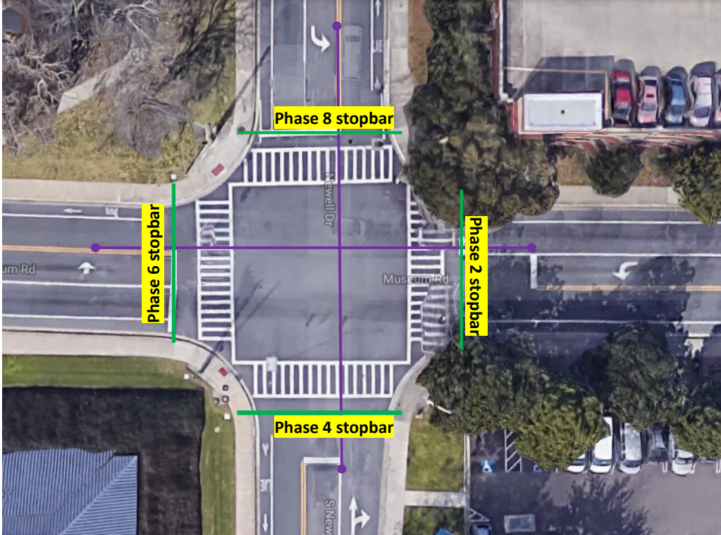
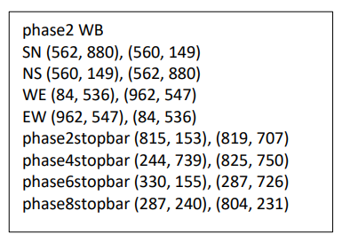
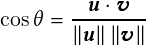
A snippet of a configuration file used to specify the reference vectors is shown in Figure 3.5. The user can specify the direction of the phase 2 movement using the phase2 parameter of this file, which has a value WB (westbound) in this example. The other phases, as described in Figure 3.1, may be derived with reference to the phase 2 direction. The parameters SN, NS, WE, and EW specify the start and endpoints of reference vectors for through lanes along south-north, north-south, west-east, and east-west directions, respectively. Figure 3.6 shows the corresponding reference vectors. The start and endpoint coordinates of the stop bars are also needed to differentiate left- and right-turn movements that otherwise align with each other. An example of this is given later in this section.
Given a trajectory, the cosine value in Equation 3.3 may be computed for the trajectory vector and the reference vectors, and if the value calculated is close to 1 for any of these vectors, the trajectory may be assigned the corresponding through a phase (one of 2, 4, 6 or 8). For any intersection, the coordinates of the reference vectors have to be determined once, and the configuration file may be reused over time until the geometry of the intersection is changed.
The next step in the hierarchical clustering scheme is to cluster the trajectories with the same movement direction. The spectral clustering algorithm is applied in this step. Prior experimentation with a simple K-means clustering approach for this problem highlights the benefits of using spectral clustering instead. A pure K-means algorithm requires user input for the number of possible clusters, which is impossible for the user to know in advance. Spectral clustering, through its smart use of standard linear algebra methods, gives the user objective feedback about possible clusters and further accentuates the trajectories’ features to make cluster separation easier.
The inputs to a spectral clustering algorithm are a set of trajectories, say tr1, tr2,  , trn, and a similarity matrix S, where any element sij of the matrix S denotes the similarity between trajectories tri and trj. It is to be noted that we consider sij = sji � 0, where sij = 0 if tri and trj are not similar. Given these two inputs, spectral clustering creates clusters of trajectories such that all trajectories in the same cluster are similar. In contrast, two trajectories belonging to different clusters
are not so similar. For example, for the given set of trajectories, spectral clustering creates separate clusters for trajectories following different lanes or those that change lanes at the intersection. As a result, spectral clustering also helps identify the outliers and anomalous trajectories that are not similar to any other trajectories in the set. The two inputs to a spectral clustering algorithm may be represented as a graph G = �V ;E�, where vertex vi in this graph represents a trajectory tri.
Two vertices are connected if the similarity sij between the corresponding trajectories tri and trj is greater than a certain threshold �, and the edge is weighted by sij. Thus, the clustering problem may be recast as finding connected components in the graph such that the sum of the weights of edges between different components is negligible. Hence, by obtaining the number of connected components, we know the number of clusters and then get the clusters by applying a K-means
algorithm.
, trn, and a similarity matrix S, where any element sij of the matrix S denotes the similarity between trajectories tri and trj. It is to be noted that we consider sij = sji � 0, where sij = 0 if tri and trj are not similar. Given these two inputs, spectral clustering creates clusters of trajectories such that all trajectories in the same cluster are similar. In contrast, two trajectories belonging to different clusters
are not so similar. For example, for the given set of trajectories, spectral clustering creates separate clusters for trajectories following different lanes or those that change lanes at the intersection. As a result, spectral clustering also helps identify the outliers and anomalous trajectories that are not similar to any other trajectories in the set. The two inputs to a spectral clustering algorithm may be represented as a graph G = �V ;E�, where vertex vi in this graph represents a trajectory tri.
Two vertices are connected if the similarity sij between the corresponding trajectories tri and trj is greater than a certain threshold �, and the edge is weighted by sij. Thus, the clustering problem may be recast as finding connected components in the graph such that the sum of the weights of edges between different components is negligible. Hence, by obtaining the number of connected components, we know the number of clusters and then get the clusters by applying a K-means
algorithm.
We used the linalg library provided by NumPy to perform the linear algebra operations in spectral clustering. Once the number k of connected components is known, a K-means algorithm is run on the first k eigenvectors to generate the clustering results. The function KMeans is a K-means clustering algorithm from the Python sklearn.cluster library.
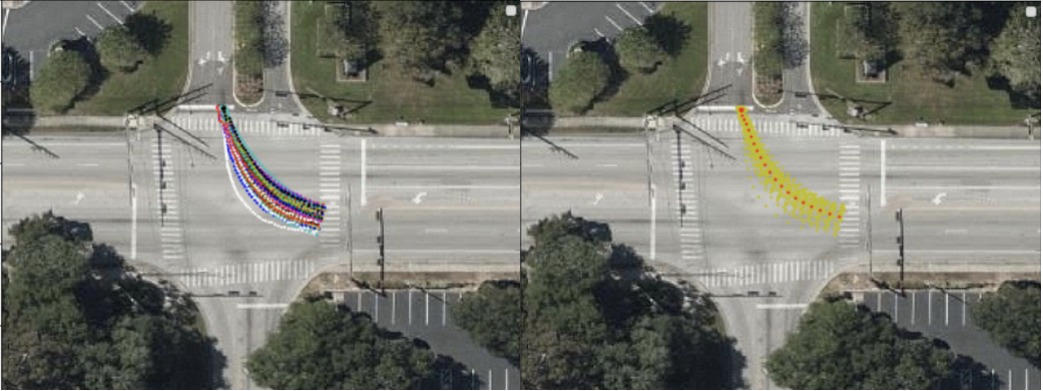
The clusters generated by spectral clustering for all the left-turn trajectories are shown in Figure 3.7. The straight and right-turn trajectories clusters are omitted here due to space constraints.


| Figure 3.7.: | Second level of the two-level hierarchical clustering scheme where spectral clustering is applied to trajectories with the same direction of motion. The clusters of some left-turn trajectories are presented in this figure. |
After the trajectories are clustered, we identify a trajectory in each cluster that is representative of that cluster. The representative for each cluster is computed as the trajectory t belonging to the cluster with the least average distance from all the other trajectories.
Detecting anomalous traffic behavior is one of the top goals for clustering trajectories. An anomalous trajectory may violate the spatial or temporal constraints at an intersection. The spatial constraints amount to the restrictions a vehicle must follow at an intersection, such as never going the wrong way. Temporal constraints, on the other hand, are the restrictions imposed by the signaling system at an intersection. We consider these two types of anomalous behavior in the rest of this section.
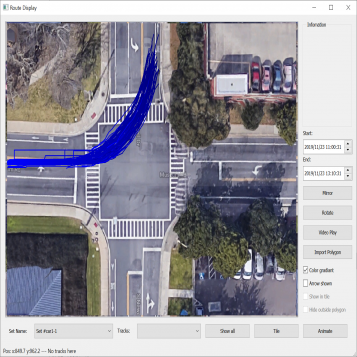
The fusion of video and signal data allows us to detect the validity of the trajectories with reference to the current signaling phase of the intersection. The video and signal clocks are sometimes off by a few seconds. Adding an offset to the trajectories may treat the clocks as synchronous. This offset may be computed manually by comparing the time a signal in the video transitions to green and the time in the signaling when there is a “Phase Begin Green” event for the corresponding phase. It is also possible to compute the offset automatically in software by checking the timestamp of the first trajectory that crosses, say, the phase 2 stop bar (Figure 3.6) and the timestamp in signal data when the phase 2 signal becomes green and then adding 2.5 seconds of driver reaction time to the signal transition timestamp. Figure 3.8 shows the trajectories during a yellow light.
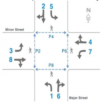
| Figure 3.8.: | Collection of tracks representing vehicles that enter the intersection on a yellow light. |
| Figure 3.9.: | Collection of tracks representing vehicles with anomalous behavior because of their shape. |
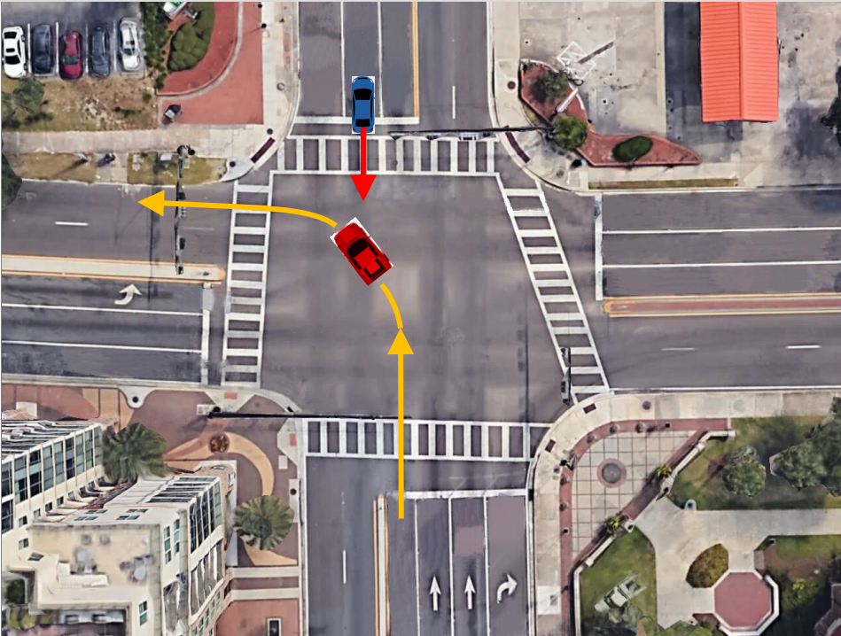
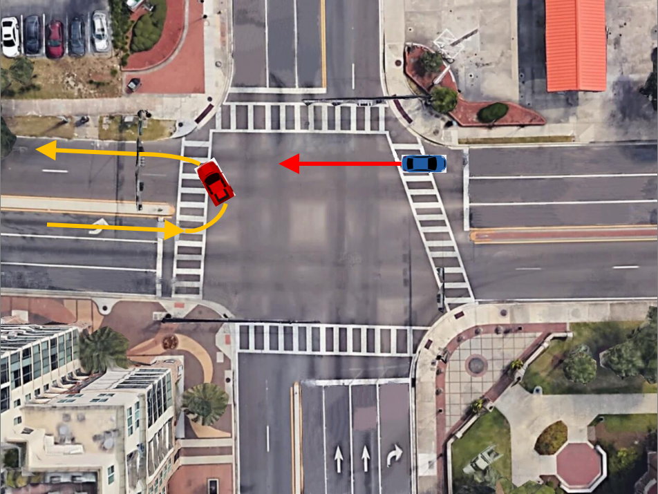
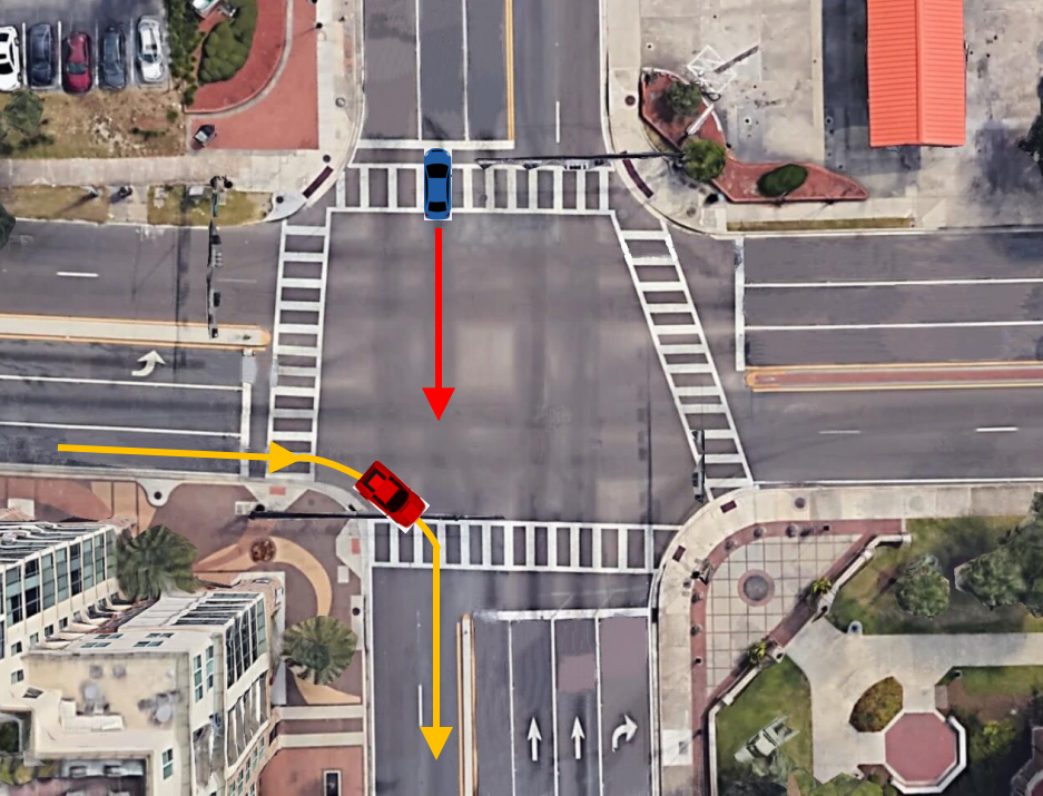
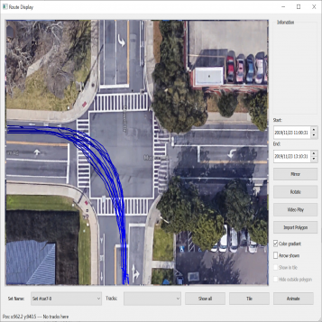
Figure 3.9 shows the anomalous trajectories. In all the cases here, the trajectories are turn movements. Sometimes these trajectories take a very wide turn. At other times, the trajectories turn left from a through lane, and at still other times, the trajectories start taking a turn much before the actual stop bar, causing wrong-way access to the adjacent lane.
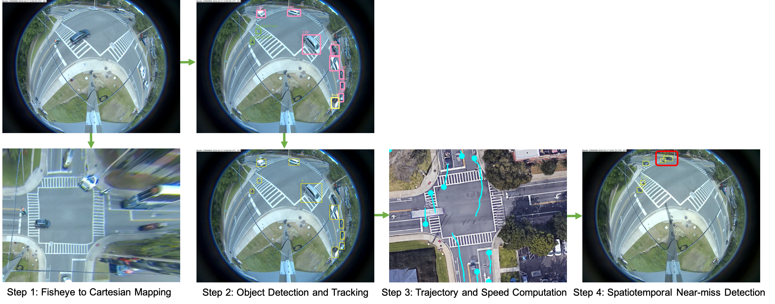
Our video processing software allows one to collect sufficient samples and visual cues corresponding to near-misses, intending to detect and even anticipate dangerous scenarios in real-time so that appropriate preventive steps can be undertaken. In particular, we focus on near-miss problems from large-scale intersection videos collected from fisheye cameras. The goal is to temporally and spatially localize and recognize near-miss cases from the fisheye video. The primary motivation for resolving distortion instead of using original fisheye videos is to compute accurate distance among objects and their proper speeds using rectangular coordinates that better represent the real world. The projections are made on an overhead satellite map of the intersection. We specify five categories of objects of interest: pedestrians, motorbikes, cars, buses, and trucks. The overhead satellite maps of intersections are derived from Google Earth�. The main steps of our detection framework (Figure 3.11) can be summarized as follows:
Figure 3.12 demonstrates the pipeline and the overall architecture of the proposed method.
Due to fisheye lens distortion and perspective distortion, we found that directly applying mapping methods between fisheye images and satellite maps does not result in good-quality mappings. Therefore, we wish to utilize fisheye camera parameters to make an initial calibration. For our fisheye camera model, points in a real 3D world are first transformed to fisheye coordinates via extrinsic parameters (rotation and translation). These fisheye coordinates are mapped into the 2D image plane via the intrinsic parameters (including the polynomial mapping coefficients of the projection function). For a point, P, in the 3D world, the transformation from world points to points in the camera reference image is:
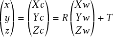 | (3.4) |
where R is the rotation matrix and T is for translation. The pinhole projection coordinates of P are �a;b� where a = x�z, b = y�z, r2 = a2 � b2, � = atan�r�. The fisheye distortion is defined as
 | (3.5) |
where the vector of distortion coefficients is �k1;k2;k3;k4� and camera matrix is
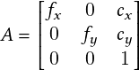 | (3.6) |
The distorted point coordinates are �x0= ��d�r�a;y0= ��d�r�b�. The final pixel coordinates vector is �u;v� where u = f x�x0� �y0�� cx and v = f yy0� cy, where skew coefficient � is set to zero and remains zero.
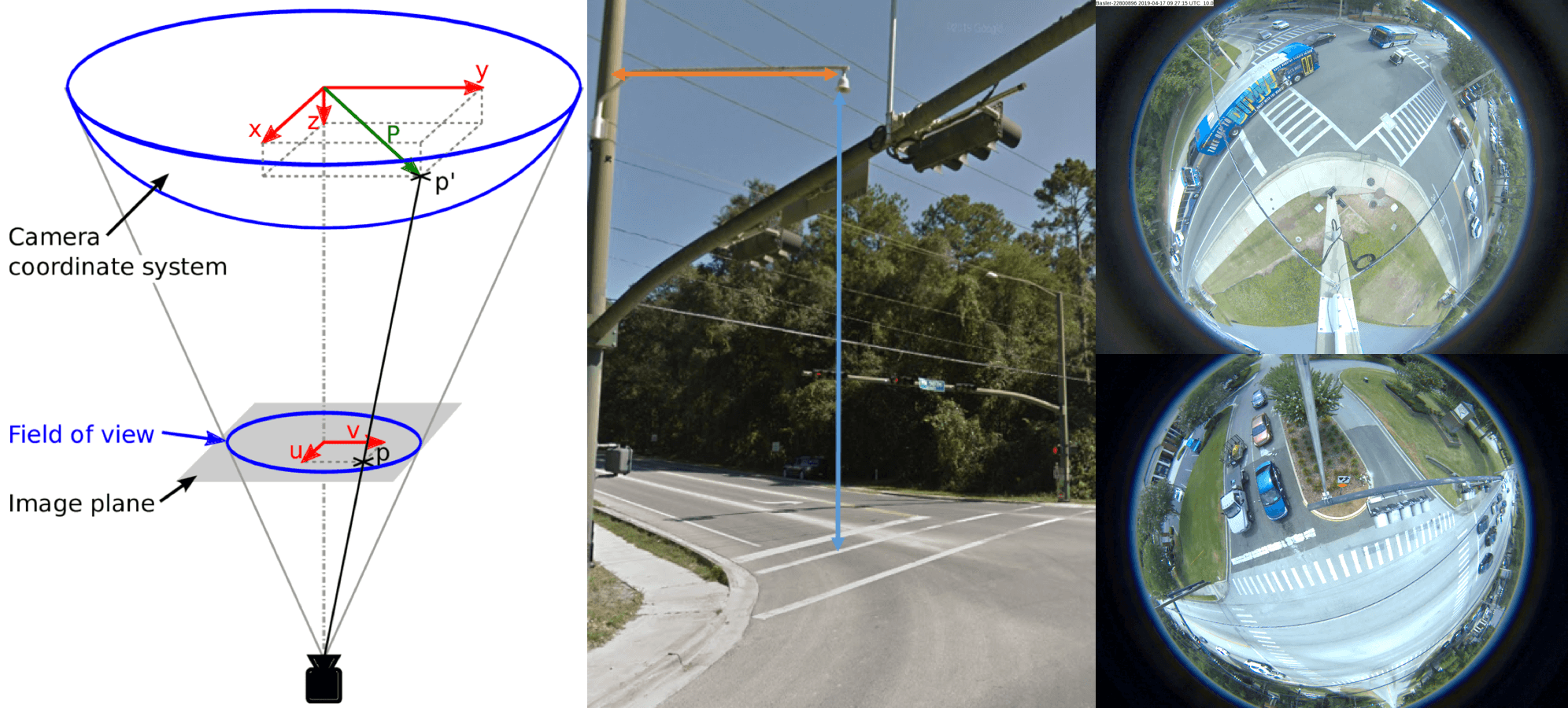
| Figure 3.13.: | An illustration of omnidirectional fisheye camera used for data collection and examples of fisheye video. |
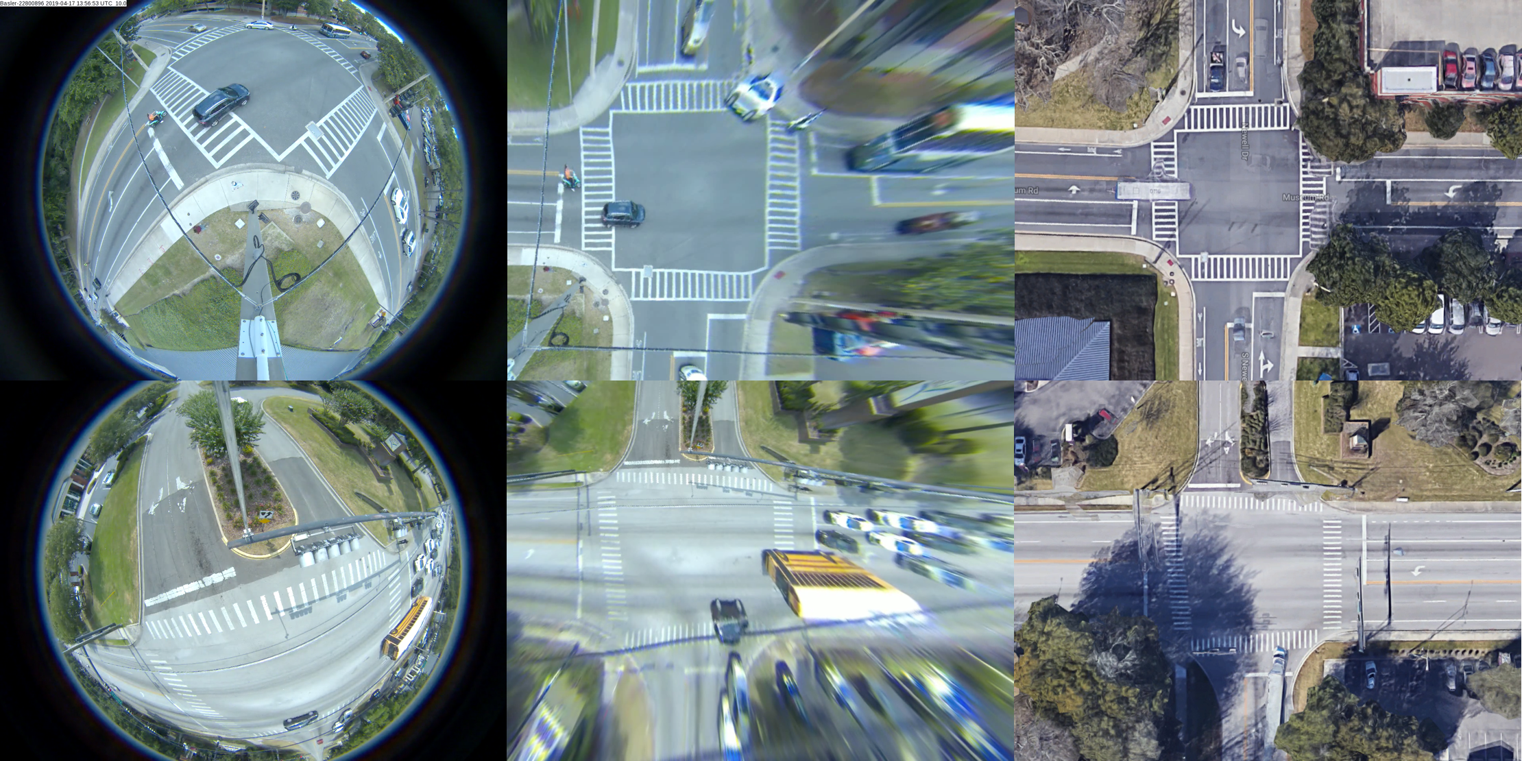
| Figure 3.14.: | Calibration and TPS mapping are used for fisheye to cartesian mapping. Left: original fisheye image. Middle: mapping result. Right: reference satellite map. |
The distortion correction procedure involves three major stages: calibration correction, perspective correction, and TPS mapping. The calibration process consists of getting parameters using a checkerboard reference. The image obtained after the calibration has a noticeable perspective distortion, which is adjusted by selecting four points in the output image of the first stage and then mapping them to a reference satellite image. There are small but noticeable distortions in the image after perspective correction caused by the structural elements of the road, such as ridges and grooves, or they may be due to minor errors caused in the calibration. The TPS mapping is used to address these distortions. In TPS mapping, multiple points are selected on the image obtained after perspective transformation and mapped to points on the satellite map. It approximates the transformation using a spline-based method. Thus by performing TPS, we get an image whose ground (road) and the map ground almost overlap. As our application goes beyond distortion correction, we can track the vehicles and get the exact location in cartesian coordinates.
After calibration and perspective correction steps, we can compute an initial fisheye to cartesian mapping. To refine the mapping between the corrected fisheye image and satellite map, we adopt the thin-plate spline (TPS) as the parameterization of the non-rigid spatial mapping connecting fisheye geometry to a Cartesian grid. The choice of TPS to handle the spatial warping in our problem is driven by the fact that it is a natural non-rigid extension of the affine map. Furthermore, we do not have any information regarding physics-based mappings that can augment fisheye calibration. Therefore, we adopt the TPS to generate mappings. Given the point sets V and Y in 2D (D = 2) consisting of points va;a = 1;2;:::;K, and ya;a = 1;2;:::;N, respectively, the TPS fits a mapping function f �x;y� using corresponding landmark sets ya and va by minimizing the following energy function [72]:
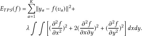 | (3.7) |
Homogeneous coordinates are used for the landmarks with each point ya represented as a vector �1;yax;yay�. With a fixed regularization parameter �, a unique minimizer, f , can be obtained as follows [72]:
 | (3.8) |
where d is a �D � 1���D � 1� matrix representing the affine transformation and w is a K ��D � 1� warping coefficient matrix representing the nonaffine deformation. The vector ��va� is a 1 �K vector related to the TPS kernel. When combined with the warping coefficients w, the TPS generates a non-rigid warping. Figure 3.13 illustrates the omnidirectional fisheye camera model, camera placement, and examples of collected video data. We present the mapping results of two intersections in Figure 3.14.
We leverage tracking results to generate a trajectory for each object in terms of frame, track ID, class, and x-y coordinates. We transform the x-y coordinates from fisheye image space to overhead satellite map space using the point-to-point mapping matrix obtained in the mapping pipeline. We estimate the speed of objects using distance after mapping. To leverage more accurate and compact object masks than rectilinear bounding boxes, we also investigate Huang et al.’s [73] use of gSLICr [22], a GPU-based implementation of SLIC [57]—a superpixel segmentation method—instead of standard rectangular bounding boxes. Figure 3.15 demonstrates the use of superpixels for generating object masks. This integration performed in real-time results in better distance measures that can be utilized for detecting near-misses.
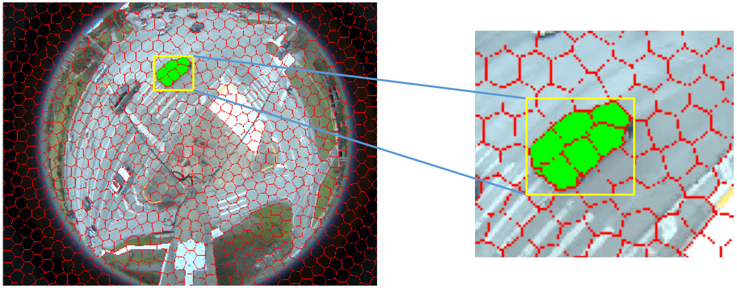
| Figure 3.15.: | An example of superpixel segmentation on fisheye video. It is used for extracting more detailed object features (with object boundaries and shapes) than detection. |
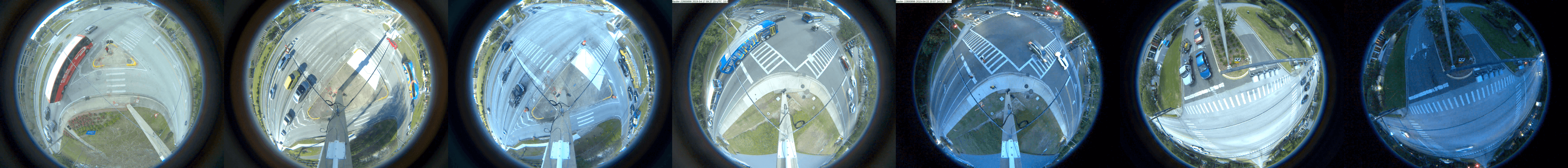
| Figure 3.16.: | Gallery images of Fisheye Video with various locations (4 cameras) and lighting conditions. |
Our method performs object detection and multiple object tracking in real time and can handle large-scale and city-scale intersection videos for traffic understanding and analysis. Using our TPS-based non-rigid mapping tool, we can correct online and offline coordinates to project road object locations to satellite maps and then form refined trajectories for near-miss detection.
Two near-miss scenarios are defined for videos: (1) spatial scenario: road objects collide or are very close in image space, and (2) temporal scenario: a dramatic speed decrease to avoid near-misses (a sudden brake). We use distance-based and speed measures to compute the near-miss probability of road objects with an average of two scores as the final output described below.
Spatial Distance Measure. We use track data to form trajectories of road objects and compute distances between two road objects using center coordinates of detected bounding boxes in image space at the frame level. The probability of a spatial near-miss is calculated using the euclidean distance of road objects with a ratio to the size of the object according to object class (vehicle size of each class does not vary much) and is computed as follows:
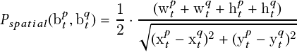 | (3.9) |
where btp and btq denote the detected bounding boxes for the p-th and q-th objects in the t-th frame. wtp, htp, xtp, ytp denote the object width, object height, x coordinate, and y coordinate for the p-th object in the t-th frame, respectively.
Temporal Motion Measure. The speed of the road object is computed by adjacent displacement over multiple time frames. The probability of motion-based near-miss is computed by the fractional decrease in speed and is computed as follows:
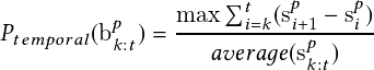 | (3.10) |
where b1:tp denotes the detected bounding boxes for the p-th from its first frame (k-th frame) to its last frame (t-th frame). sip denotes speed for the p-th object in the i-th frame. We use a weighted average of the above two probabilities of near-miss to compute the overall score.
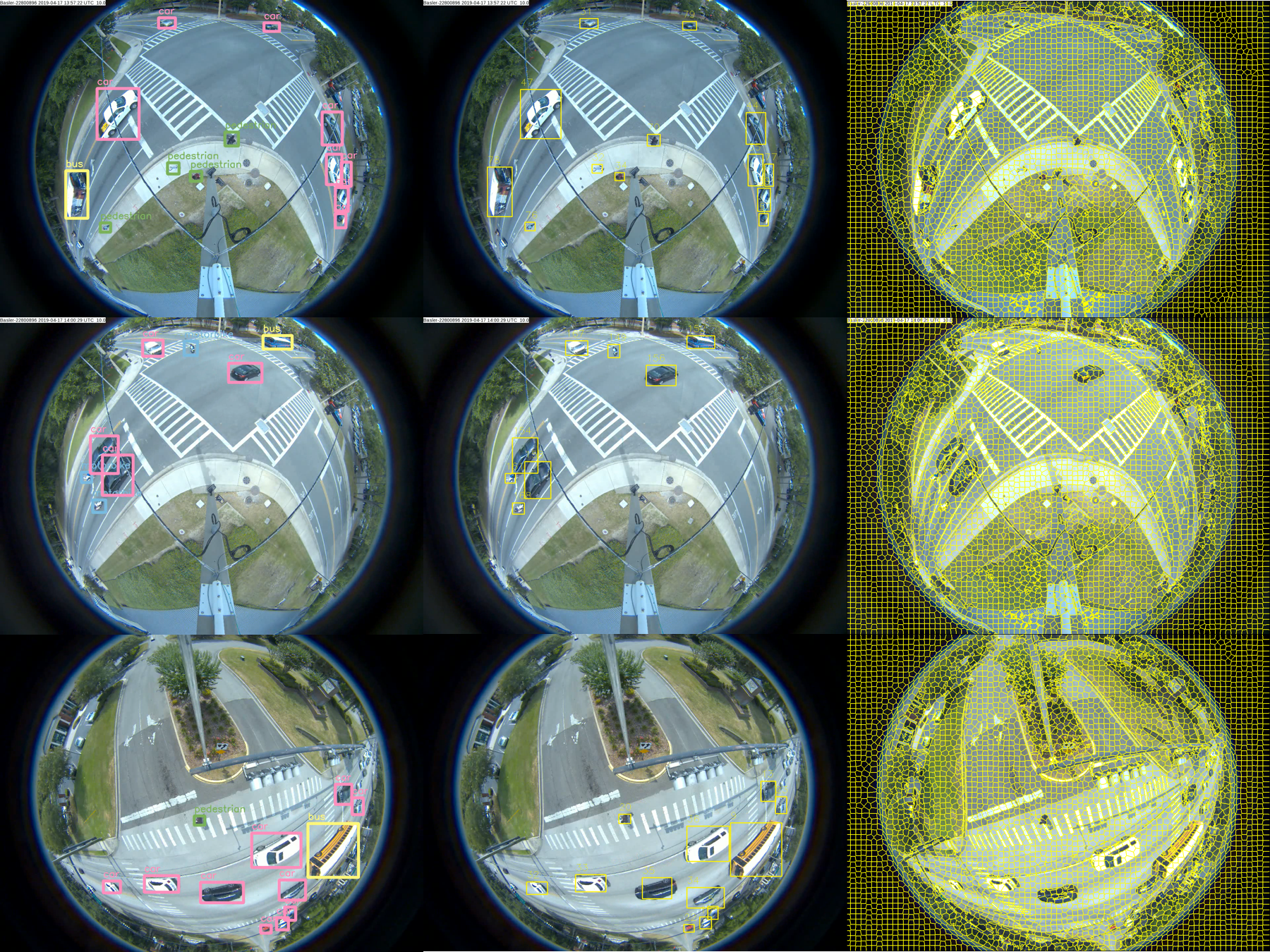
| Figure 3.17.: | Qualitative results of detection, tracking, and segmentation tasks. Left: object detection outputs the object class (car, pedestrian, bus, motorbike, etc.) and localization (bounding box). Middle: multiple object tracking associates the object in consecutive video frames (track ID). Right : superpixel segmentation aids in computing object boundaries and shapes. |
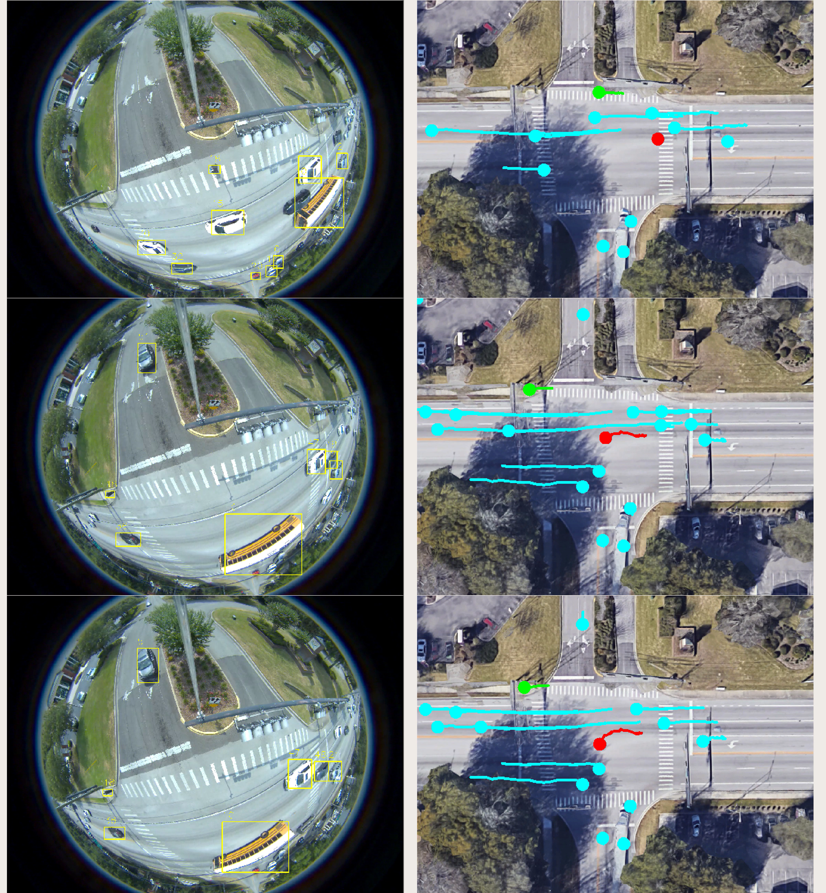
| Figure 3.18.: | Qualitative results of object trajectories mapping to satellite map. Left: tracking in fisheye video. Right: trajectories after mapping. Different color represents different object class (red for bus, green for pedestrian, and blue for car). |
We first describe the dataset used for our experimental evaluation. We then present qualitative performance and quantitative assessment of our methods for object detection, multiple object tracking, superpixel segmentation, thin-plate spline, and near-miss detection. We present a performance comparison between a non-mapping-based method and our proposed calibration+TPS-based method for near-miss detection.
We have collected large-scale fisheye traffic video from omnidirectional cameras at several intersections. Figure 3.16 shows gallery images of the dataset with several collected fisheye video samples at multiple intersections under different lighting conditions. We collected 8 hours of videos daily for each intersection: 2 hours each for the morning, noon, afternoon, and evening. The total video datasets used in the experiments have a duration of more than 100 hours. As discussed earlier, fisheye intersection videos are more challenging than videos in other datasets collected by surveillance cameras for reasons including fisheye distortion, multiple object types (pedestrians and vehicles), and diverse lighting conditions. We manually annotated the spatial location (bounding boxes) and temporal location (frames) for each object and near-miss to generate ground truth for object detection, tracking, and near-miss detection. We also annotated the corresponding vehicle class.
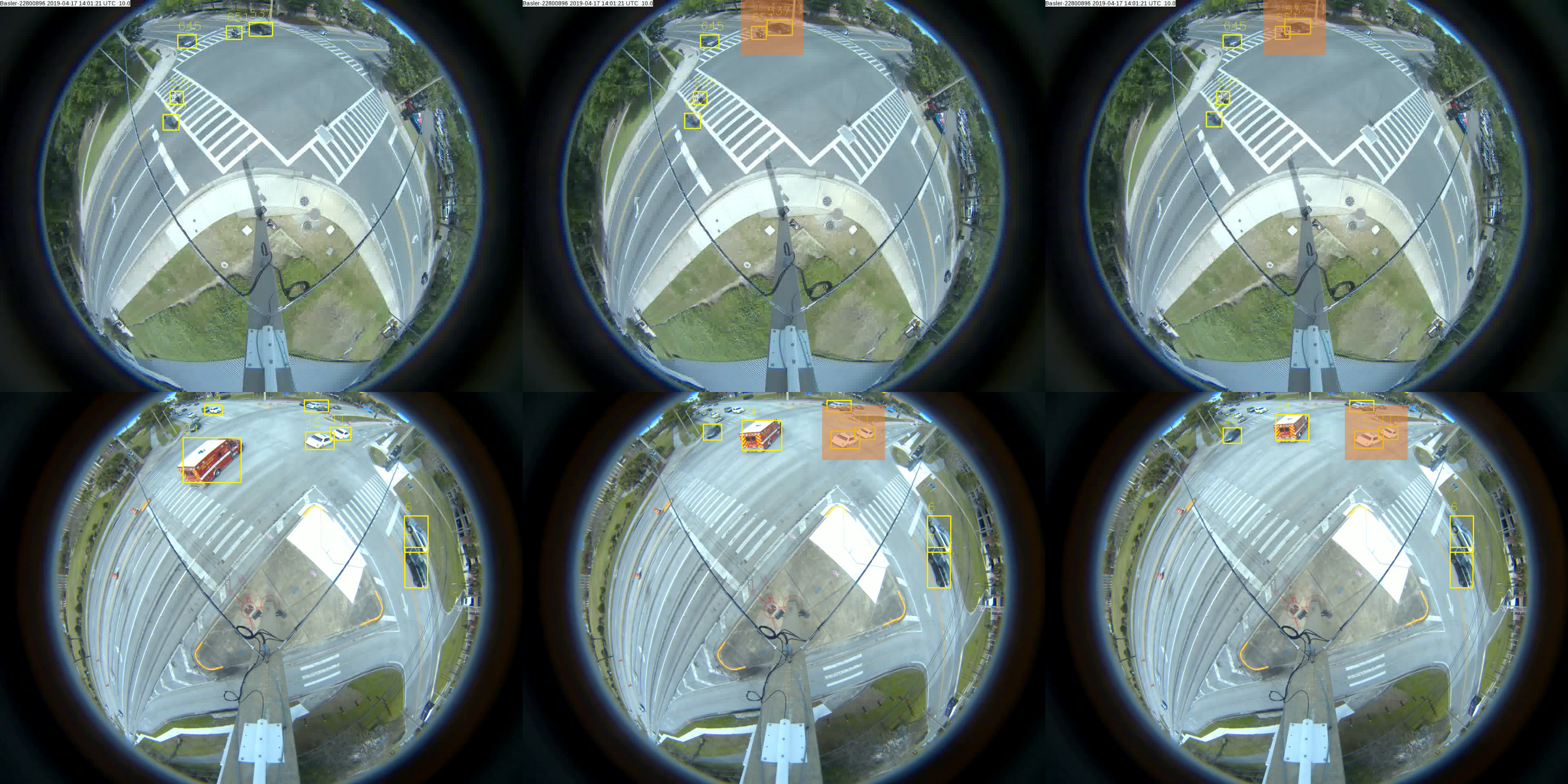
| Figure 3.19.: | Qualitative results of two types of near-miss detected. Top 3 images: a spatial near-miss case: a motorbike and a car collide. Bottom 3 images: a temporal near-miss case caused a sudden brake. |
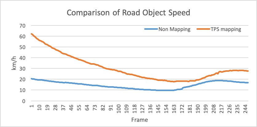
| Figure 3.20.: | Quantitative comparison of computed object speed between non-mapping and proposed methods. |
| Table 3.3.: | Quantitative comparison of near-miss detection between non-mapping and calibration+TPS-based method. |
The results for the calibration+TPS pipeline (Figure 3.14) show that fisheye distortion and perspective distortion are effectively addressed by our method. The qualitative results in terms of performance for object detection, multiple object tracking, and superpixel segmentation (Figure 3.17) show that the deep learning-based detector is effective in classifying objects even when the image footprint is small (e.g., pedestrians and motorbikes). The use of deep cosine metric learning allows the tracker to generate more consistent and stable tracks. The superpixel segmentation assists in outputting compact contours of objects. The latter can then be used for an effective signature for tracking.
The trajectories of road objects projected on the satellite map, along with referenced tracking frames, are shown in Figure 3.18. These trajectory maps give an easier-to-understand traffic pattern for the intersection than that from the perspective of the original fisheye camera. Samples of near-misses that we detected at different intersections are presented in Figure 3.19. The first example shows a spatial near-miss between two road objects. The second example shows a temporal near-miss as the front white car suddenly stopped in the middle of the intersection, forcing a sudden brake for the following vehicle.
We present a quantitative evaluation of the overall performance of our proposed method in terms of speed performance, improvement of object speed measures based on mapping, and the precision and recall for each subtask of the pipeline.
We present the speed performance for the tested methods in Table 3.1. The fisheye video resolution is 1280 � 960, and our implementation for thin-plate spline takes 10 s for one-to-one corresponding mapping for 1,228,800 points. This is a one-time setup cost.
After getting mapping point sets, all video processing experiments were performed on a single GPU (NVIDIA Titan V). The GPU-based SLIC segmentation [57] has excellent speed and can process 400 fps on fisheye videos. The overall pipeline of our methods (object detection, multiple object tracking, and near-miss detection) achieves about 40 fps. This rate is sufficient to address a variety of real traffic surveillance and near-miss detection for large-scale daily video data.
A quantitative prediction of object representation and near-miss is achieved by comparing predicted detection with the ground truth at the frame level. A true positive corresponds to a high level of overlap between the prediction and ground truth detection pair. It is computed using an Intersection over Union (IoU) score. The track is correctly associated if this overlap exceeds a predefined threshold (e.g., 0.7). A true negative means no prediction and no associated ground truth. A false positive is that a prediction has no associated ground truth. A false negative is that a ground truth has no associated prediction. The true negative rate (TNR) also refers to specificity, and the false positive rate (FPR) refers to fallout. The specificity, fallout, precision, recall, and F1-score are defined as
 | (3.11) |
 | (3.12) |
 | (3.13) |
We compute object speed information based on trajectories by converting pixels to actual meters and frame intervals to seconds. Figure 3.20 shows an example of the comparison of computed object speed information where a car approaches the intersection with speed decreasing from 60 km/h to 20 km/h and then back to 30 km/h. With non-mapping methods, object speed computing suffers from fisheye and perspective distortion and yields inaccurate results. We also present accuracy evaluation for object and multiple object detection (cosine metric learning) in Table 3.2. As real near-miss is rare in terms of two-camera video data in a week, it is more reasonable to examine specificity (selectivity or true negative rate) and fallout (false positive rate) for near-miss detection. In Table 3.3, we present the comparison of non-mapping-based detection and calibration+TPS mapping-based detection in terms of true negative rate (TNR) and false positive rate (FPR). The quantitative evaluation demonstrates the overall effectiveness of our proposed method for near-miss detection in large-scale fisheye traffic videos.
Using a deep learning model integrated with camera calibration and spline-based mapping methods, we presented a novel unsupervised approach to detect near-misses in fisheye intersection video. It maps road object coordinates in fisheye images to a satellite-based overhead map to correct fisheye lens and camera perspective distortion. This allows for computing distance and speed more accurately. This unified approach performs real-time object recognition, multiple object tracking, and near-miss detection in fisheye video. Handling geometry on object-level analysis in the fisheye video is efficient and robust, resulting in more accurate near-miss detection. The experimental results demonstrate the effectiveness of our approach, and we show a promising pipeline broadly applicable to fisheye–video-understanding applications such as accident anticipation, anomaly detection, and trajectory prediction.
As we get rich spatial and temporal features of road objects in both fisheye image space and overhead satellite image space, these track data can be easily applied to several other traffic and computer vision tasks such as anomaly detection, trajectory clustering, trajectory prediction, turn movement counts, etc. Intersection signal data can be integrated with video data to develop interesting traffic analyses, e.g., cars crossing the intersection during a red light. The generated tracks can be plotted over extended periods (shown in Figure 3.21) to visualize macro trends.
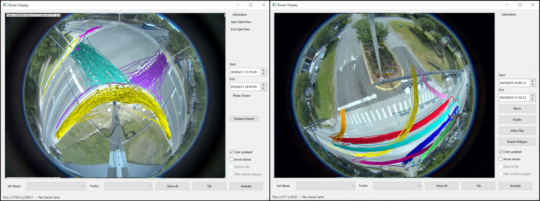
| Figure 3.21.: | An example of trajectory visualization used in our visualization tool. Left: pedestrian trajectories in intersection 01. Right : vehicle trajectories in intersection 02. Color means different clusters after clustering. |
Intersection safety is an active area of research because traffic intersections are prone to crashes. USDOT estimates more than 50% of road crashes leading to fatality or injury happen at or near traffic intersections. Road crashes have been one of the leading causes of death worldwide. With the rapid advancement in technology, many intersections now have video cameras deployed as sensors to monitor these intersections. The videos are streamed over the Web, stored, and processed for safety assessment. Existing intersection safety assessment methodologies often require the analysis of historical data to infer current and future intersection user behavior. Although helpful, these data are often biased to what has been reported, incomplete, and retrospective. This chapter will present our end-to-end intersection safety methodology, starting with processing intersection videos and computing existing and new “surrogate safety measures.”
Based on decades of safety research using crash data, it is generally acknowledged that using surrogate safety measures could provide further insights into enhancing the safety of roadways. These surrogate measures rely on maneuvers (trajectories) of vehicles and pedestrians. Countermeasures can be developed to reduce or eliminate unsafe maneuvers by understanding trajectories that could have led to a crash. The most common surrogate safety measure is the “near-miss” or the “traffic conflict.” Near misses involve a vehicle’s trajectory coming very close to that of another vehicle or a pedestrian without an actual collision. The proximity of the trajectories is measured on a temporal scale using metrics such as time-to-collision (TTC) [74], and post-encroachment time (PET) [75]. The severity of the near-miss event can be determined based on the temporal proximity measures (TTC and PET) and the velocities of the vehicles or pedestrians involved. Typically, shorter TTC and PET, combined with higher relative speeds, imply a greater severity of the near-miss (i.e., the lesser likelihood of not avoiding the potential crash and higher injury severity had the crash not been avoided). Unlike the case of crashes, there are currently no clear thresholds or categories for classifying near-misses by severity. In this chapter, we introduce a new surrogate safety measure, “severe event,” that includes all near-miss events and unsafe behavior exhibited by road users.
While surrogate safety measures offer an excellent opportunity to understand site-specific and time-specific safety issues and develop countermeasures, a tremendous practical impediment in using surrogate measures for safety analysis is the need to process large volumes of video data to determine trajectories, identify the conflicts in these trajectories, and filter these down to a subset of critical unsafe maneuvers for further analysis. In signalized intersections, it is also necessary to analyze the unsafe maneuvers for the ongoing signal phasing data to identify the appropriate countermeasures. For example, unsafe maneuvers during a permitted left-turn phase may suggest the need for a protected left-turn phase. Similarly, conflicts between right-turning vehicles and crossing pedestrians may suggest separating the signal phases for these two movements (no right turn on red or leading pedestrian phase). This chapter makes several contributions to the field of intersection safety analysis, described as follows:
We have applied our algorithms to multiple intersections in two different cities. Our extensive results demonstrate the usefulness of the software by providing key insights into severe conflicts by the day-of-the-week and hour-of-the-day analysis.
The rest of the chapter is organized as follows. Section 4.2 presents the related work in traffic safety analysis using surrogate safety measures. Section 4.3 presents the overall methodology we developed, starting with trajectory generation and computation of features from the trajectories, our strategy of classification of serious conflicts, and the introduction of the new surrogate safety measure, severe event that we developed as a part of this work. We present a set of event filters to filter out events that are not potentially dangerous automatically. Section 4.4 presents our experimental results, and we conclude in Section 4.5.
Several surrogate safety measures have been developed, relying on the physical properties (time, distance, and speed) of vehicle trajectories. Measures such as TTC and PET, which are based on the temporal proximity of the road users, are perhaps the most widely used indicators, especially in the context of intersections, which are the focus of this chapter. TTC is the time remaining to avoid a collision, from when the road user takes action to where the collision can occur [74]. PET is the time difference between when the first road user leaves one point and when the second road user arrives at that same point [75]. Lower values of TTC and PET indicate higher risks of collision. Several other measures have been proposed based on either spatial proximity or acceleration-deceleration patterns of vehicles [76, 77]. A very comprehensive synthesis of the literature on surrogate safety measures was recently provided by Arun et al. [78].
Just as all traffic crashes are not equally severe (some could lead to fatalities while a vast majority are minor crashes with only property damage but no injuries), all temporally proximal interactions among road users need not be “safety-critical” events. Even though Hydn [79] proposed over three decades ago that there is a hierarchy of traffic events varying in severity, Arun et al. [78] note that there is still no consensus on what constitutes a safety-critical event or a near-miss.
One approach to identifying critical events is applying thresholds on surrogate safety measures. For example, thresholds on TTC range from 1.5 to 3.0 seconds [80, 81], while those for PET range from 1.0 to 1.5 sec [82]. Broadly, the perception-reaction time of road users (the time taken by a road user to understand a situation and react to it) is considered a benchmark in determining these thresholds.
surrogate safety measures primarily reflect the possible interactions (or “events”) between road users; not all are critical from a safety standpoint. Therefore, it is essential to distinguish between safer and critical interactions. Safety-critical events are also known as near-misses or sometimes as traffic conflicts, but the definition of a traffic conflict has remained contentious over years [78]. The early definitions of traffic conflicts indicate that only the most extreme traffic interactions have been considered safety critical. Hydn [79] proposed a hierarchy of traffic events varying in severity. Arun et al. [78] note that there is still no consensus on what constitutes a safety-critical event or a near-miss.
A second approach to identifying critical conflicts is the Swedish Traffic Conflict Technique [83]. This approach considers both the surrogate measure and the speed of the conflicting road users. In general, events representing a combination of lower times to crash and a higher conflict speed are considered more serious events. Figure 4.1 presents an example of conflict curves. Vehicle-vehicle conflicts above curve 26 are considered serious, while vehicle-pedestrian conflicts above curve 24 are considered serious [84].
Determining surrogate safety measures and critical safety events requires trajectories of road users (vehicles and pedestrians) as inputs. These trajectories may be obtained from traffic simulators or the processing of real-world video data. The Surrogate Safety Assessment Model (SSAM) has been developed as a post-processor to estimate the number and severity of conflicts based on vehicle trajectory data [84]. The outputs of SSAM include the number, the type, the severity, and the locations of three types of simulated conflicts (crossing, lane changing, and rear-end). The conflict type is identified according to the lane and link information or the angle between the two converging vehicles.
Commercial applications for processing trajectory data from videos to determine surrogate measures include those developed by DERQ, AMAG, Currux, and Transoft Solutions. Our work in this chapter is closely related to McLauchlan et al. [85], where the authors use video analysis for intersection traffic analysis. The main difference is that [85] has not treated pedestrian-vehicle conflicts. Further, only PET was used as a safety indicator. In contrast, we use a holistic approach to compute and use PET and TTC (as appropriate), speed, deceleration, and distance between the road users as active features for severe-event detection. These features give a deeper insight into the event’s nature and get us nearer to the events that are indeed close calls.
The methodology used for this work is described as follows. Section 4.3.1 presents the salient features generated by our software to qualify the events and their use for safety analysis. Section 4.3.2 introduces a new surrogate safety measure, severe event, and describes a categorization scheme for vehicle-vehicle and pedestrian-vehicle events. Section 4.3.3 describes a filtering process, an event sieve that helps narrow down the events to keep only the most critical events. Finally, Section 4.3.4 describes a multi-attribute decision tree approach to isolate high-intensity regions in feature space containing the most severe events.
Trajectories are generated by processing the intersection videos. The safety analysis system takes fisheye video footage as input, then annotates objects with bounding boxes, maps those coordinates from the fisheye image to rectilinear space, and then stores the results in the trajectory table. The object detection and tracking module utilizes YOLOv4 [86] to detect different kinds of road participants, including vehicles, pedestrians, cyclists, and motorcyclists. A modified deepsort algorithm associates detections across frames and assigns a unique ID for each object. As the trajectories from fisheye videos are usually of unnatural shapes caused by lens distortion, we perform rectification and alignment to Google Maps images before feeding the trajectories to downstream modules. Our solution for rectification includes two steps: fisheye-to-perspective transformation followed by thin-plate spline (TPS) warping.
Separately, the city’s Automated Traffic Signal Performance Measures (ATSPM) data are collected, which provides the signal information for each traffic light per intersection over time. This signal information is merged with object trajectories, enabling analyses concerned with object location and signal states over time, such as signal violations, lingering mid-trajectory, etc. However, one issue that arises is the synchronization of city-provided and video-recorded signal changes, which usually vary by a few seconds. A purpose-built computer vision model is trained to output signal states, which are compared to ATSPM signal changes to yield the time delay between video and city data. If a signal is not visible, then the start-up time of a vehicle is used under the assumption that driver reaction time is roughly one and a half seconds, but this time is configurable in the software.
We have computed a comprehensive set of features for every conflict event. A feature in this context is an individual measurable property or characteristic of a conflicting event. The following is a list of the key features that we compute:
Figure 4.2 shows the intersection labels for the crosswalks that will be used throughout the book.
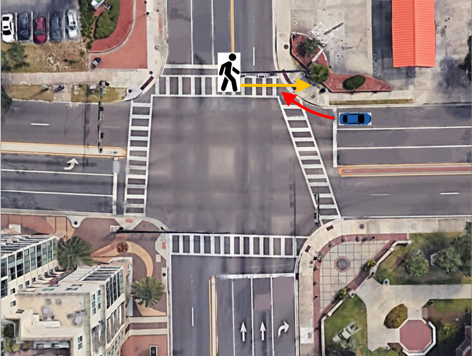
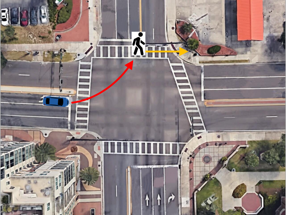
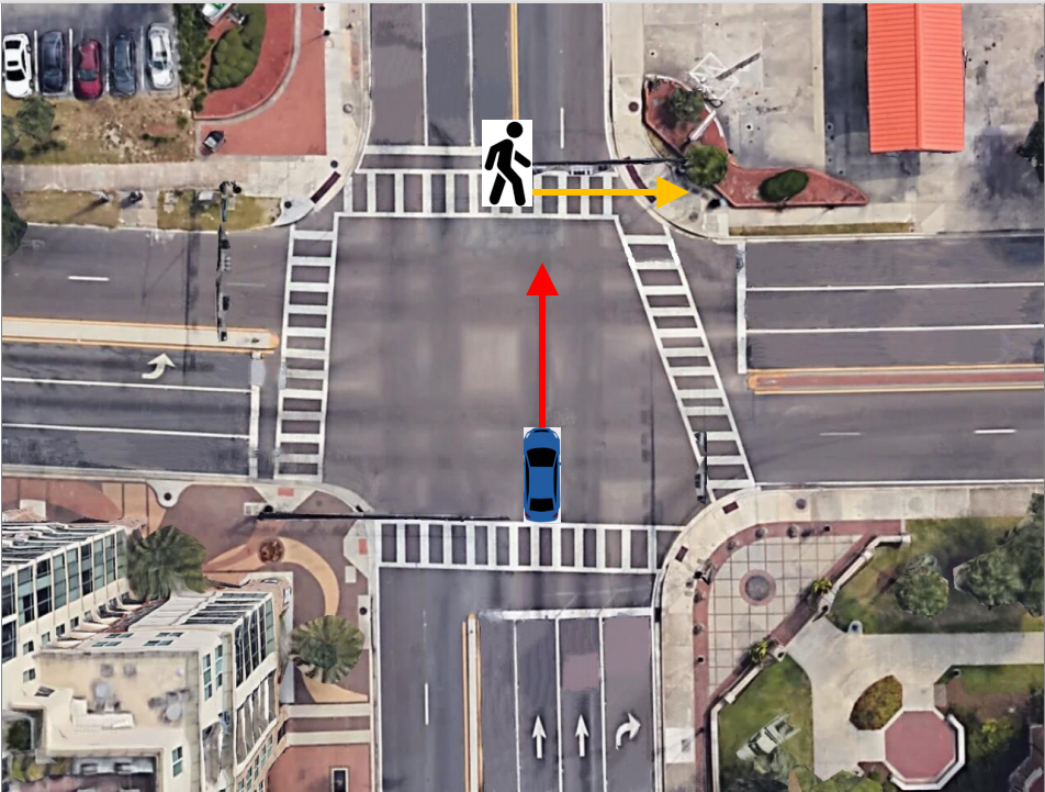
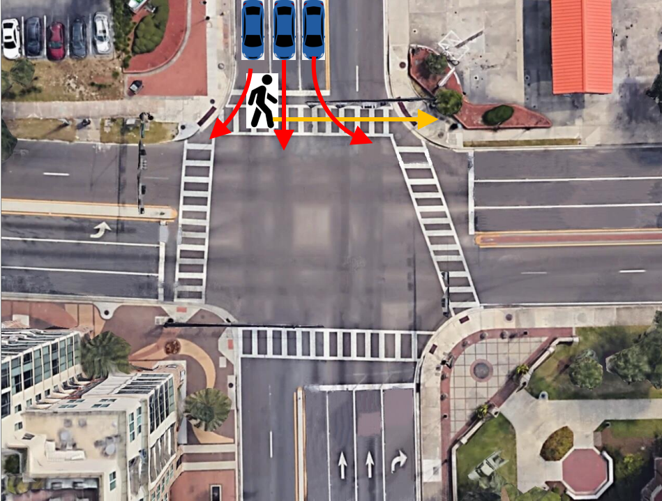
| Figure 4.3.: | P2V conflict types. |
The categorization of the vehicle-vehicle and pedestrian-vehicle conflicts is described in this section.
Among these conflicts, Conflict Types 1 and 3 are possible conflicts between pedestrians and vehicles at signalized intersections if all vehicles and pedestrians strictly follow the traffic rules (assuming a three- or four-leg intersection, which are the most common).
If one or more vehicles do not strictly follow traffic rules (e.g., run the red light), other conflicts are also possible, namely, adjacent through movements, left turn, and adjacent through. Some conflict types may be inherently more dangerous than other types. For example, the left turn and opposing through conflicts may lead to a more serious crash than a merging, a diverging, or a rear-end conflict. Further, the left turn and opposing through conflict is dangerous when the slow left-turning vehicle is the first to cross the conflict point. The less dangerous and common occurrence is when the left-turning vehicles yield to the through vehicles before completing the turn.
Figure 4.5 shows the multistage event filter we employ to prune the set of events. The macrofiltering stage checks the following conditions for two road users at the intersection in the same time frame: (1) Are they in a conflicting traffic phase? (2) Is the TTC or PET within a user-defined threshold, say, 10 seconds? (3) Are they spatially within or close to the intersection and within a user-defined threshold, say, 10 meters from each other? and (4) Are both road users moving?
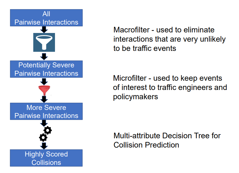
| Figure 4.5.: | Event filtering sieve. The macrofilter checks for movement phases of conflicting trajectories, timing, and distance features. The microfilter checks finer aspects, such as whether yields were properly given. |
The event passes through to the microfilter when all these conditions are satisfied. The first check for vehicle-vehicle interactions in the microfilter is whether an event is recorded more than once from separate TTC and PET computations. If the event did not result in a post-encroachment and there is no corresponding PET, the event must last for more than one decisecond to be considered severe. The second check for vehicle-vehicle interactions is whether each vehicle properly yielded to the other as per the traffic rules in case of a conflicting movement. If so, the event is filtered away.
For pedestrian-vehicle interactions, the first check in the microfilter is to find if the pedestrian is violating the pedestrian signal. If so, the event is considered severe, even if no vehicles are nearby. Highlighting the behavior allows practitioners to be aware of a pattern and adjust signal timing if needed. Suppose the pedestrian follows the signal, yet the event already made it through the macrofilter (indicating a conflicting maneuver); in that case, the microfilter checks if the distance between the pedestrian and the vehicle is 5 meters or less. If so, then the event is considered severe. On the other hand, if the pedestrian is about to enter the crosswalk and the vehicle is close by, the filter checks if the pedestrian’s distance is less than 1 meter, and in that case, the event is considered severe.
All the thresholds mentioned in this section are easily configurable by the user based on specific intersection geometry and user characteristics.
Although the event filters were efficient in pruning the event set, manually reviewing the filtered videos still constitutes a significant investment of human resources. For this reason, we utilize a simple algorithm to determine high-intensity regions in the feature space for severe events, where these events have been annotated manually. Because the event count after applying the filters is small compared to the total number of features for the events, there is a high chance of overfitting if a feature space with all the features is considered. So, to determine the high-intensity regions, we use only three features: speed, acceleration, and TTC or PET, as appropriate for that event. The algorithm plots 2D scatter plots of the events for each pair of features from the three-feature set and then sweeps the 2D space with a straight line to find the best intercept for which the line separates the severe and the non-severe events. The straight line acts as a separator of the 2D feature space, and we consider several such lines with different slopes to arrive at a near-optimal partitioning. This process is repeated for each partition if a partition is not purely from one class of events and contains a good mix of severe and non-severe events. In any case, the process is repeated up to a maximum of three levels of recursion. This algorithm could lead to more than one high-intensity region for the same dataset, which, once identified, can be conveniently used as a classifier for severe events. An example is presented in the experiments section. Human ratings of events are used to validate the model’s predictions.
We applied our video processing algorithms end-to-end on six different intersections for the first week in November 2021. We collected data between 6 AM and 7 PM for each intersection, yielding 546 hours of video data, which were processed using our software and analyzed for intersection safety. Table 4.1 gives the intersection details. Based on video analysis, Table 4.1 also presents the total traffic and the percentage of pedestrians versus drivers. Three intersections are on an arterial adjacent to a university (ID: 1, 2, 3), one intersection is adjacent to a high school (ID: 4), and the two other intersections are in a city (ID: 5, 6). Though all these intersections have right-hand-drive traffic, our algorithms can also analyze intersections with left-hand-drive traffic.
We present our results on conflict analysis separately for pedestrians and vehicles in Sections IVA and IVB, respectively. While Table 4.1 gives an aggregate volume of the total number of pedestrians observed during the study period, we can further disaggregate the pedestrian count by the pedestrian phases and by day of the week and hour of the day. We present this analysis for the intersection of University Ave & 13th Street, but the other intersections may be analyzed similarly. Four pedestrian phases, P2, P4, P6, and P8, and eight vehicle phases, 1-8, for the University Ave & 13th Street intersection are shown in Figure 4.6.
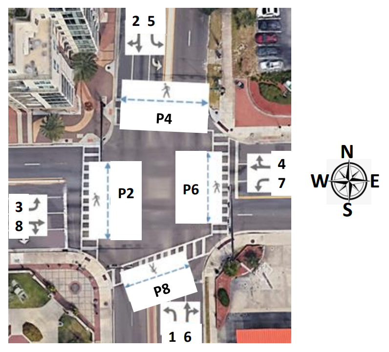
| Figure 4.6.: | Four pedestrian phases, P2, P4, P6, and P8, and the eight vehicle phases, 1, 2, 3, 4, 5, 6, 7, and 8, are shown for University Ave & 13th St. |
Figure 4.7 shows the pedestrian volumes for the four pedestrian phases at the University Avenue & 13th Street intersection by day of week and hour of the day. We observe that (i) the volume in phase 4 is the highest, (ii) the volume on a Saturday, November 13, 2021, is the highest because there was a football game at the university stadium on University Avenue, (iii) the volumes on Monday and Tuesday are higher than the rest of the weekdays, and (iv) this intersection is large, so the pedestrians on the closest crosswalks are the best processed by the video processor. The crosswalks may be ordered as phases 4, 2, 6, and 8 by their proximity to the camera.
Figure 4.8 counts pedestrian-vehicle conflicts by the conflict type and cycle on the University Avenue & 13th Street intersection. The conflicts are shown by the day of the week and the hour of the day. We observe: (i) Conflict Type 1, which is a right-turning vehicle with a pedestrian on the adjacent parallel crosswalk, occurs most frequently; (ii) Conflict Type 1 happens throughout the day but is more likely to happen around 12-2 PM; (iii) Conflict Type 3, which is a left-turning vehicle with a pedestrian on the parallel opposite crosswalk, happens most frequently on game day; (iv) Conflict Type 5, which is a through vehicle with a pedestrian on the far crosswalk, a dangerous conflict, happens more frequently during 1-4 PM. The vehicular movements can further analyze each conflict type, and Figure 4.9 shows a sample of such an analysis. We observe that the afternoons and weekends are when pedestrians are more prone to violate the traffic light and undertake dangerous crossings. For Conflict Type 1, we found that the westbound right (WBR) and southbound right (SBR) happen most frequently on weekdays and weekends. Such detailed analysis of pedestrian-vehicle conflicts could give insights into countermeasures to reduce conflicts.
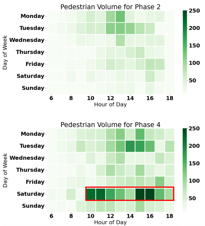
| Figure 4.7.: | Pedestrian volumes by the four pedestrian phases at the University Avenue & 13th Street intersection. Among the weekdays, Monday and Tuesday are busier at this intersection. On Saturday, November 13, 2021, pedestrian traffic was especially high because of a football game being held at the University Stadium. |
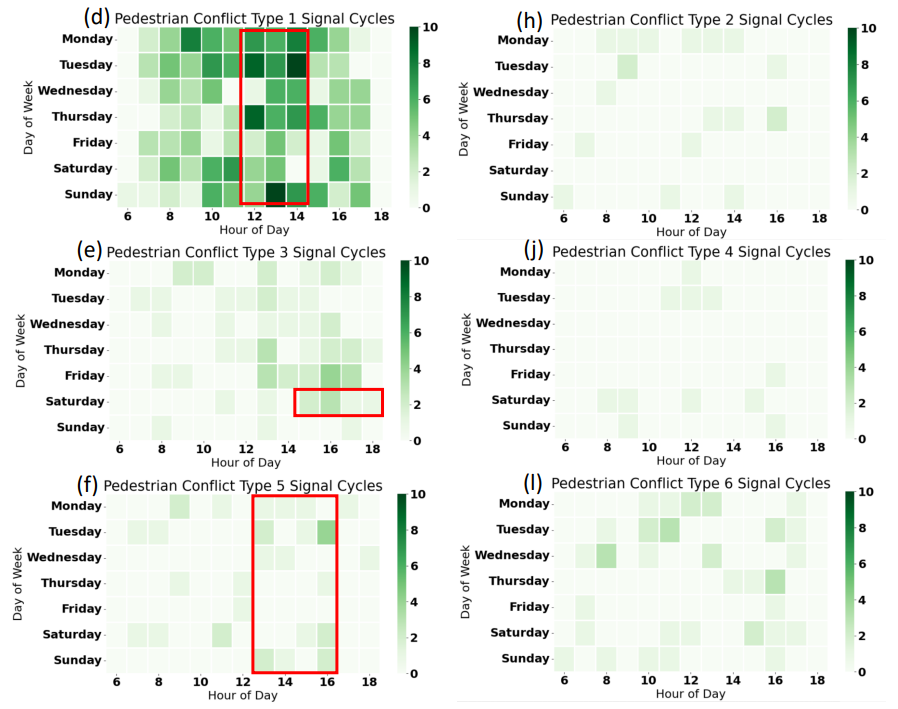
| Figure 4.8.: | The pedestrian-vehicle conflict events are categorized into six conflict types and counted by day of the week and hour of the day. Figures (a), (b), and (c) give the raw event count for Conflict Types 1, 3, and 5, while figures (d), (e), and (f) give a count of signal cycles with at least one conflict. Conflict Type 1 occurs most frequently and is more likely between 12 and 2 PM. Saturday, November 13, 2021, was a game day, and there was an uptick in the conflict counts from (c). However, these conflicts are clustered, and fewer signal cycles are affected, as can be seen from (d), Conflict Type 5, which is through vehicle with pedestrians in the far crosswalk, a dangerous conflict that happens more frequently during 1-4 PM. |
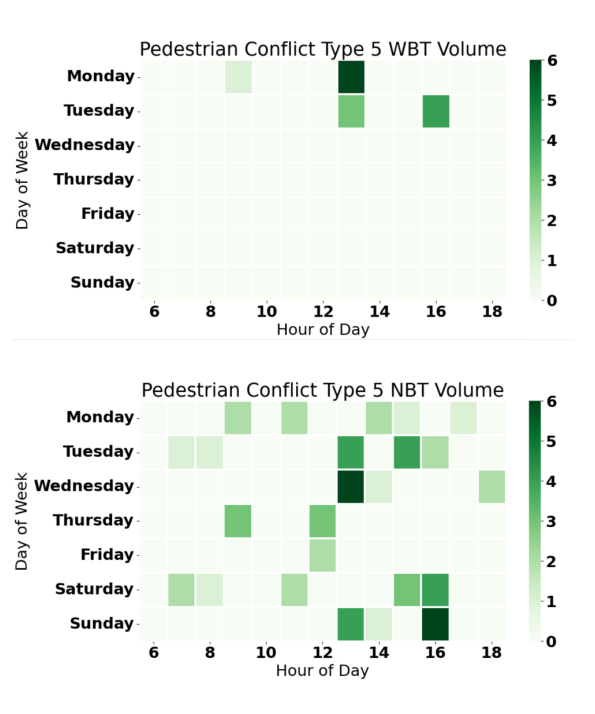
| Figure 4.9.: | Volume of pedestrian-vehicle Conflict Type 5 by vehicle movement. This conflict type is the most dangerous between a through vehicle and a pedestrian in the far crosswalk. We have watched the video in almost all these cases and found that pedestrians violate their signals. |
Table 4.2 shows the number of potentially conflicting interactions over a week and the performance of the two-level macro- and microfilters in filtering the events.
| Table 4.2.: | Total number of potentially conflicting interactions over a week from different intersections and performance of the two-level macro- and microfilters in filtering the events to a handful for further manual analysis. After applying our multi-attribute decision tree algorithm, the column V2V MADT contains the event counts. |
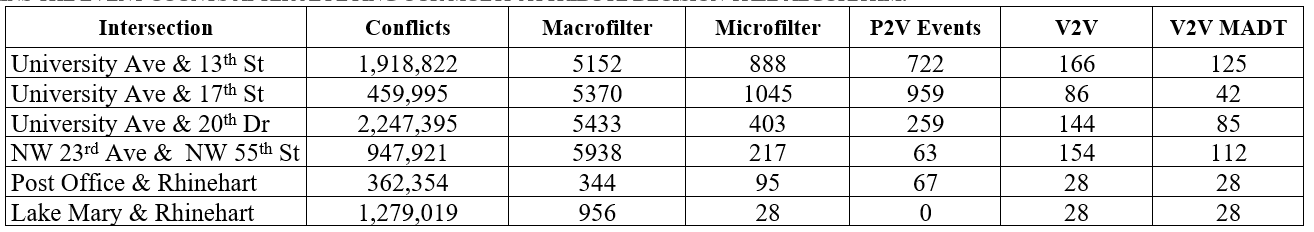
The events include both vehicle-vehicle and pedestrian-vehicle conflicts. All pedestrian-vehicle events that remain after applying the microfilter are considered severe by default because of the vulnerable nature of pedestrians.
We manually verified for vehicle-vehicle events that 30% to 60% of these might be regarded as severe. We further applied our multi-attribute decision tree algorithm for classifying an unseen event automatically as severe or non-severe. The results of this step are presented in the Vehicle-Vehicle Multi-Attribute Decision Tree (V2V MADT) column that further reduces the count of severe events, which may be quickly evaluated manually for insights into applicable countermeasures. Thus, starting from millions of potential conflict interactions, our filtering scheme reduced the events to a small set of severe events.
| Table 4.3.: | Vehicle-to-vehicle conflicts: (a) Total sum; (b) Weighted sum (relative weight of 4 assigned to left opposing through); (c) Normalized based on exposure (per 10,000 vehicles) |
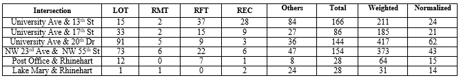
Table 4.3 categorizes the vehicle-vehicle conflict types into the previously defined classes. Some conflicts did not belong to any of our defined conflict types. Among the known conflict types, left opposing through is the most severe as it could lead to significant damage to life and property if any of the conflicts results in a collision. The other conflict types are merging, or diverging conflicts, and any resulting collision yields a very low-impact crash. So, event categorization helps emphasize only the more dangerous conflict types by placing more weight on them. For example, in Table 4.3, the column titled “Total” is a simple sum of all conflict types, whereas the column titled ”Weighted” gives a weighted total, where the left opposing through conflicts have been assigned a weight of 4. The “Normalized” column computes the conflict volume per 10,000 road users. These numbers are obtained by dividing the weighted conflicts by the corresponding exposure metric (explained in the next paragraph) and multiplying by 10,000. The “Normalized” conflicts allow us to rank the intersections by safety. For example, we can conclude from Table 4.3 that the Lake Mary & Rhinehart intersection is the safest. Table 4.4 shows the exposure metrics for the known conflict types. The exposure metric was computed as the sum of the number of vehicles participating in either of the two movements involved in a conflict. For example, if there is a conflict between northbound left (NBL) and southbound through (SBT), then the exposure metric for left opposing through will have a component that is the sum of all vehicles making NBL and SBT maneuvers. The exposure metric serves as a denominator in normalizing the conflict volume. Figure 4.10 shows the steps in our algorithm for isolating the high-intensity regions in the three-dimensional space of (maxSpeed, maxDeceleration, minTime). For a conflict, maxSpeed defines the maximum speed of the two vehicles involved, while maxDeceleration is the maximum brake applied by either of the two vehicles. minTime is the minimum time for TTC or PET, which comes from the point representation of the involved vehicles and a bounding box representation of these vehicles. We take the minimum of these two times. The data used in Figure 4.10 are from the NW 23rd Ave & NW 55th Street intersection. The steps in the algorithm are demonstrated in Figure 4.10(a-d). The high-intensity region is obtained from randomly processing 80 of 100 filtered events from the intersections. The remaining 20 events are used to test the classifier. We manually annotated the 100 filtered events as severe or non-severe. The accuracy of this scheme is 90%, with a 92% recall and 90% precision. We used our algorithm separately for each intersection. The splits shown in Figure 4.10 are different for each intersection because the intersections have other characteristics such as speed limits, a school nearby, etc. The column V2V MADT in Table 4.2 shows the volume of events that were further pruned by our algorithm to find high-intensity regions. We did not apply the MADT algorithm to P2V events because pedestrians are vulnerable users, and all conflicts that remain after using the filters are considered severe by default. The accuracy of the MADT algorithm depends on the accuracy of video processing algorithms because video processing plays a crucial role in the computation of the safety features such as speed and deceleration.
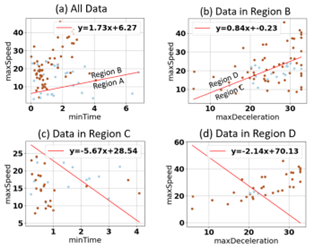
| Figure 4.10.: | The steps in finding high-intensity regions of severe events. (a) All data and the line that separates them. In this diagram, the red dots represent severe events, while the blue dots represent non-severe events. The data here are from the NW 23rd Avenue & NW 55th Street intersection. Region A consists of non-severe points. (b) Region B is further split into regions C and D. Splitting regions C and D again, in (c) and (d), respectively, gives us high-intensity regions. |
This chapter developed a systematic and novel methodology for analyzing intersection safety based on video analysis. We developed algorithms that use video analysis and signal timing data to perform accurate event detection and categorization in terms of the phase and type of conflict for both pedestrian-vehicle and vehicle-vehicle interactions. We introduced a new surrogate safety measure, severe event, quantified by multiple metrics such as TTC or PET as recorded in the event, deceleration, and speed. We developed an efficient multistage event filtering approach followed by a multi-attribute decision tree approach that prunes the extensive set of conflicting interactions to a robust set of severe events.
Using our analysis and based on the limited number of intersections, we found that the dominant conflicts at intersections with heavy pedestrian use are right-turning vehicles on the adjacent parallel crosswalk. We could identify the specific right-turn directions contributing to this problem and the hours during the week when the problem peaks. Categorization of vehicle-vehicle interactions showed that for intersections with permissive left turns, the more common conflict is between a left-turning vehicle and an opposite-through vehicle. The intersections with protected left-only displayed some merging and diverging conflicts, inherently less severe.
Intersection safety studies are essential because traffic intersections are prone to crashes leading to injury or fatality [87]. According to USDOT, more than 50% of road crashes leading to fatality or injury happen at or near traffic intersections. With rapid technological advancement and price drops [88], video cameras are now commonly deployed as sensors in traffic intersections. Existing intersection safety assessment methodologies often require the analysis of historical data to infer current and future intersection user behavior. Although helpful, these data are often biased toward what has been reported, which is retrospective and often incomplete. Video analysis of traffic intersections has no reporting or survivorship biases because the analysis times from the fisheye camera [89] are precise and unbiased. This chapter presents a methodology to systematically use the trajectory data from video analysis, severe events data, and signal phasing data to detect and analyze conflict hotspots and evaluate the efficacy of countermeasures to improve intersection safety. The trajectory and severe events data are available from our previous work [90], which implemented video processing and severe event detection algorithms. The signal phasing data are available from the advanced traffic controllers (ATC) at traffic intersections.
We present a novel evaluation engine. The engine ingests trajectory data, severe events data, and signal phasing data at a given intersection for different days of the week and times of the day.
The evaluation engine has three primary data processing modules: the first module computes pedestrian and vehicle volume hotspots; the second module computes pedestrian-vehicle (P2V) and vehicle-vehicle (V2V) conflict hotspots; the third evaluates intersection service as a proxy to intersection performance for the study period. Multiple signal phasing configurations may be systematically analyzed using the evaluation engine to develop volume and conflict heatmaps and a performance-safety tradeoff chart for the intersection. Traffic engineers may use this tradeoff chart to select a configuration that optimizes intersection safety and performance.
More detail is presented below about the three primary data processing modules:
The evaluation engine with the modules above may be used for studying performance-safety tradeoffs from multiple signal-phasing configuration scenarios. We can analyze the current scenario using the evaluation engine and arrive at an appropriate countermeasure to potentially improve safety or performance issues at the intersection. We demonstrate the operation of the evaluation engine on two different intersections using more than a week of data on each intersection. One of these intersections is near a high school with teenage pedestrians and drivers. The other intersection has a pedestrian presence of more than 40% of the total users.
The key contributions of this chapter are described as follows:
The rest of the chapter is organized as follows. Section 5.1 presents the related work while Section 5.2 presents the background for work. Next, Section 5.3 presents our system’s in-built methodology and how we can use it systematically to discover and address safety issues. Section 5.4 illustrates how to apply the steps to find the safety issues for both pedestrian-vehicle (P2V) and vehicle-vehicle (V2V) interactions at two different intersections. Finally, we discuss the key findings in Section 5.5.
traffic intersections are more at risk for near-miss events and accidents. This section first describes surrogate safety measures: what and how they are beneficial. The sensors available today to compute the surrogate safety measures are discussed next, and finally, the existing work on traffic safety analysis using video processing is presented.
Surrogate safety measures are indicators that strongly correlate to traffic conflicts [93, 94]. Surrogate safety measures effectively detect near-miss events, which occur much more frequently than crashes and are generally not reported through traditional channels. Crash analysis studies require years of data because of the infrequent nature of actual traffic collisions [95, 96]. Combined with the fact that crash data are often incomplete due to the under-reporting of crashes and injuries and that the geometry of the intersection may change over such long periods, the effectiveness of crash analysis studies diminishes significantly. Surrogate safety studies, on the other hand, can uncover important safety issues using about a week of video footage, making it a time and cost-effective solution for monitoring traffic intersections.
The surrogate safety measures most commonly used for near-miss detection are time-to-collision (TTC) and post-encroachment-time (PET). TTC is the time remaining to prevent a collision (by applying brakes, steering away, or using some other preventive action), measured precisely as the difference between the time the road user takes action to the point where the collision can occur [74]. PET is the difference between when the first road user leaves a point and the second road user reaches that point [75]. Lower values of TTC and PET indicate higher risks of collision [97]. After computation of TTC and PET, one way to identify severe events is by applying thresholds on TTC and PET [85, 98]. Several other proposed measures are based on either spatial proximity or acceleration-deceleration patterns of vehicles [76, 77, 78]. Our software considers TTC and PET (thresholded values) with other measures such as speed, acceleration, and distance between the two road users when a severe event happens. The thresholds we use are 2 seconds for TTC and 3 seconds for PET. These values are configurable so that the user can set them to different ones. The early definitions of traffic conflicts indicate that only the most extreme of traffic interactions have been considered safety critical [99]. Hyden [79] proposed a hierarchy of traffic events varying in severity. Arun et al. [78] note that there is still no consensus on what constitutes a safety-critical event or a near-miss. Vogel [100] compares headway and TTC as safety indicators, showing that these two measures are independent. Peesapati et al. [101] evaluated and found that PET is effective as a surrogate measure for a left turn and opposing through conflicts. Feng et al. [102] found a strong correlation between factors leading to near-misses and those leading to crashes, which highlights the benefits of analyzing the surrogate safety measures for severe near-miss events.
Johnsson et al. [103] find surrogate safety measures appropriate for vulnerable road users, including pedestrians and bicyclists. Fu et al. [104] developed a framework for assessing the safety of pedestrian-vehicle interactions. Chen at al. [105] developed lane-based models for evaluating pedestrian-vehicle interactions at non-signalized crosswalks.
After fusing surrogate safety measures with crash analysis data, Yang et al. [106] created a new surrogate measure, risk status. Surrogate safety measures are also used extensively in traffic simulation models [93, 107] and connected autonomous vehicles [108, 109].
loop detectors [110] are traditionally installed at intersections for monitoring traffic and signaling states. While these detectors are very effective in detecting traffic incidents [111], it is not possible to get the exact location of the conflict from these under-the-ground detectors. With recent technological advancements, various sensors, such as video, lidar, and infrared (IR) cameras, are being used for intersection monitoring [12, 112, 113].
Video-based traffic monitoring is increasingly popular because it is relatively low-cost and fast to process and analyze [114]. Unlike data from loop detectors, video footage gives us rich information about the object trajectories, object classification (e.g., car, bus, truck, motorcycle, pedestrian), precise location and severity of traffic conflicts, and traffic violations. Unlike lidar and IR cameras, video cameras are easier to deploy and maintain [115]. Video data are also easier to review and understand than lidar and IR camera outputs. On the downside, video cameras depend on proper lighting conditions at intersections. The two main types of video cameras are ordinary cameras and fisheye cameras. The advantage of using fisheye cameras is that a single camera can monitor the whole intersection for smaller intersections, and two cameras are sufficient for the slightly bigger ones. On the other hand, with ordinary cameras, a traffic intersection would require as many cameras as there are approaches (typically 4) to monitor the intersection completely [116].
The viability of video cameras for traffic monitoring has encouraged the development of robust video processing algorithms and surrogate safety measures. Hence, intersection safety assessment using video analysis is an active research topic. We will briefly review the existing work in this area. We reuse the video processing framework developed in our previous paper [90]. Section 5.2 provides the details of our video processing algorithm.
The differences between this work and our previous work [90] are as follows. The software [90] was used for processing the videos and generating a database of trajectory data and severe events over multiple days of the week and times of the day. In this chapter, we develop an evaluation engine that uses the trajectory, severe events, and signal phasing data to perform a spatiotemporal analysis over multiple intersections to identify temporal conflict hotspots and volume hotspots. This chapter presents a visual representation of P2V and V2V conflicts that annotates heatmaps with symbols that give the practitioner clues about the spatial locations of the conflicts and the movements of the involved trajectories for further analysis. Additionally, the evaluation engine determines overall performance and safety metrics for a given signal phasing configuration scenario and plots a performance-safety tradeoff chart for an intersection for multiple scenarios. Such a chart would be helpful to a traffic engineer for the selection of a countermeasure because it would give an idea of the performance safety characteristics of that or similar configurations.
This section presents a collection of existing work on traffic intersection monitoring using video cameras [117]. Ultimately, we compare the current work to two other recent papers on safety assessment using video analysis.
Saunier et al. [118] developed a framework to estimate collision probabilities and their spatial distributions based on video data collected in Kentucky. Ismail [119] treats the use of computer vision techniques to process traffic video data for intersection safety analysis. Stipancic et al. [120] develop and evaluate the crash frequency and severity models, incorporating GPS-derived surrogate safety measures as predictive variables. St-Aubin [121] developed a thesis studying computer vision techniques for traffic roundabouts.
Our work is closely related to the work by Samara et al. [85], where the authors use video analysis for analyzing intersection traffic. The main difference is that the work [85] has not treated P2V conflicts. Further, we can identify trajectories that help to pinpoint any persistent issues with specific movements. Moreover, the work [85] uses only PET as a safety indicator and does not discuss phase-based conflict hotspots for conflicts. Neither is there a treatment for countermeasures to improve intersection safety nor how intersection safety impacts intersection performance.
Kronprasert et al. [122] study safety performance using a video-based traffic conflict analysis system. They do not use fisheye cameras but rather regular ones that monitor the direction they point to, which requires multiple cameras. Moreover, the videos from all the cameras must be merged to get complete information about the intersection trajectories. Furthermore, the surrogate safety measure used [122] was TTC only. Our work presented in this chapter considers P2V conflicts. For P2V and V2V conflict hotspots, we do a more advanced level of conflict categorization regarding the involved trajectories.
Given a video captured by a fisheye camera at an intersection, there are six steps in our video analytics system: process the footage to extract trajectories that are timestamped �x;y� coordinates; fuse the trajectories with signaling information; process the trajectories to mine features that help with safety analysis; find all P2V and V2V conflict events; filter the events to retain only the “severe events”; and categorize the event based on the involved trajectories. These steps have been presented previously [90] and are included here for completeness.
With a fisheye video as input, the video analysis software draws a bounding box around each object in a video frame, identifies the object’s class based on several previously annotated images, and finds the �x;y� coordinates of the object as the center point of the bounding box. A video frame is a static snapshot. The fisheye cameras installed at the intersections capture 10 video frames per second. The object detection and tracking module utilizes YOLOv4 [123] to detect different road participants, including cars, buses, trucks, pedestrians, and motorcyclists. A modified deepsort algorithm [52] associates detections across frames and assigns a unique ID for each object. The �x;y� coordinates are in the circular fisheye space. A fisheye lens has a wide angle, creating a panoramic or hemispherical nonrectilinear image. So we apply a post-processing step to map the coordinates to rectilinear space using fisheye-to-perspective transformation followed by thin-plate spline (TPS) warping [124, 125, 68]. The new timestamped coordinates in the rectilinear space are stored in a database (DB) table.
The high-resolution controller logs [126] provided by the appropriate agency are analyzed to extract signal phasing information for an intersection. Fusing the signal phasing with object trajectory coordinates over the time axes gives us a holistic view of a trajectory based on when the object arrived and left the intersection. We use this information later to count the vehicles that pass the stop bar in any one direction in intervals of five seconds after the traffic light turns green.
The following is a list of the key features we compute:
The categorization of the P2V and V2V conflicts is described in this section and used in the rest of the chapter.
1. P2V conflicts: The following are the main conflicts between vehicles and pedestrians at signalized intersections:
Among these conflicts, Conflict Types 1 and 3 are possible conflicts between pedestrians and vehicles at signalized intersections if all vehicles and pedestrians strictly follow the traffic rules (assuming a three- or four-leg intersection, which are the most common).
2. V2V conflicts: As the primary purpose of signalization is to reduce or eliminate conflicting movements at the intersection, the following are the possible conflicts between vehicles at signalized intersections if all vehicles strictly follow the traffic rules (assuming a three- or four-leg intersection, which are the most common):
If one or more vehicles do not strictly follow traffic rules (e.g., run the red light), other conflicts are possible, namely, adjacent through movements, left turn, and adjacent through. Some conflict types may be inherently more dangerous than the other types. For example, the left turn and opposing through conflicts may lead to a more serious crash than a merging, a diverging, or a rear-end conflict. Further, the left-turn and opposing through conflicts are more dangerous when the slow left-turning vehicle is the first to cross the conflict point. The less dangerous, relatively common occurrence is when the left-turning vehicles yield to the through vehicles before completing the turn.
Using trajectory data and severe events from multiple videos over different hours of the day and days of the week, we compute temporal volume and find conflict hotspots. The spatiotemporal analysis helps discover safety issues in the intersection and when and where they occur. This knowledge is crucial for arriving at effective countermeasures with minimal impact on the rest of the traffic.
Figure 5.1 shows our evaluation engine and the various engine modules with their inputs and outputs. The evaluation engine modules are described in detail below.
The volume hotspot detection module is the first module of the evaluation engine that estimates (1) pedestrian volume on the different crosswalks and (2) volume peaks and troughs by the time of day and day of the week. For example, this module will help answer a query such as “How many pedestrians crossed using the north crosswalk leg of intersection X between 12 PM and 1 PM?” or “When does pedestrian volume aggregated on an hourly basis exceed a threshold T on intersection X for a given period Y?” Thus, the pedestrian hotspot detection module exposes the times of day when the pedestrian volume peaks and provides a guideline to a traffic engineer about the time of day when countermeasures for alleviating potential P2V conflicts may be implemented. Usually, such countermeasures penalize intersection performance, so implementing such countermeasures in targeted time intervals instead of throughout the day may benefit pedestrians and vehicles.
Similarly, the vehicle hotspot detection module may be used to compute vehicle volume. In contrast to video cameras, the loop detectors installed in the intersection cannot distinguish between through and right-turning vehicles. The vehicle hotspot detection module exposes times of the day and days of the week when the vehicle volume peaks for a given movement. The volume hotspot detection module could output turning movement counts (TMC) for all movements over user-selected time intervals. For example, the module can output the total number of vehicles with movement NBT, NBL, NBR, SBT, SBL, SBR, EBT, EBL, EBR, WBT, WBL, and WBR, every 15 minutes during the AM peak.
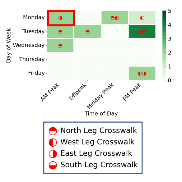
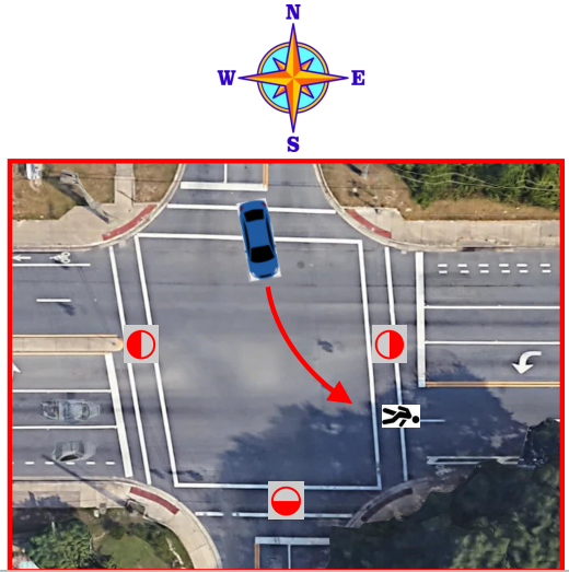
| Figure 5.2.: | The spatial location of P2V conflicts is overlaid on the heatmap. Given the P2V conflict type, one can derive the trajectories from the overhead view of the crosswalk (b). |
The second module in the evaluation engine computes the temporal hotspots of P2V and V2V conflicts and the conflict types. Examples of conflict types are, for P2V, a left-turning vehicle with a pedestrian on the far-side [parallel opposite] crosswalk (Figure 5.2b), and for V2V conflicts, a left-turning vehicle conflicting with an opposing through vehicle (LOT, Figure 5.3b). Section 5.2.4 lists conflict types in the “severe event” database.
This chapter develops a visualization scheme to describe the spatial location where conflicts happen in the intersection. This is illustrated in Figures 5.2 and 5.3. Given the conflict type and the quadrant information, it is possible to derive the movements of the trajectories involved in the conflicts. For example, for the P2V conflict chart in Figure 5.2a, there are a few conflicts on the east crosswalk during Monday’s AM peak. Since the type of the P2V conflict is a vehicle turning left with a pedestrian on the far-side [parallel opposite] crosswalk, we can derive the vehicle movement as SBL, as illustrated in Figure 5.2b.
Similarly, the V2V conflict chart in Figure 5.3a shows a LOT conflict in the SW quadrant on Monday’s midday peak. This implies that the movements of the conflicting trajectories are WBL and EBT, as demonstrated in Figure 5.3b. If a specific combination of phases emerges repetitively from this analysis, the traffic engineer could selectively address those. Otherwise, a countermeasure that impacts all phases must be applied if all phases have similar conflicts. Discovering such patterns is crucial for arriving at effective countermeasures.
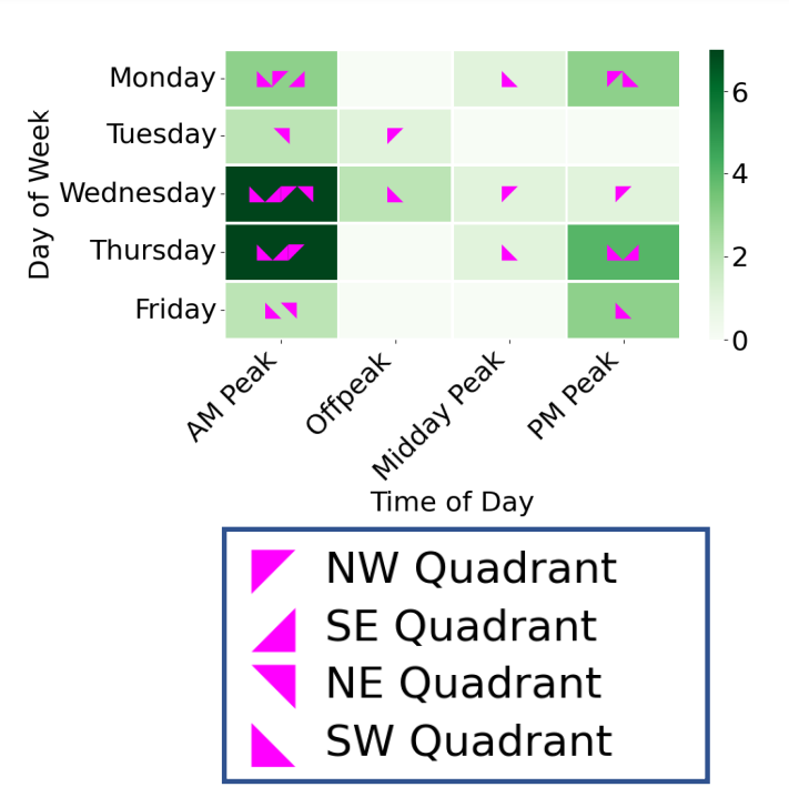
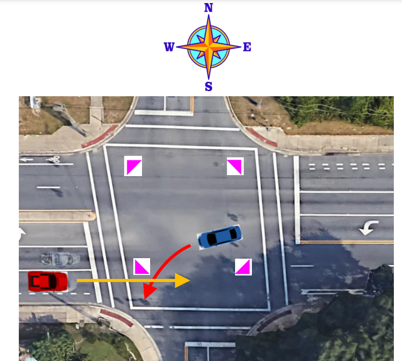
| Figure 5.3.: | The spatial location of V2V conflicts is overlaid on the heatmap. Given the V2V conflict type, one can derive the movements of the trajectories from the quadrant as shown in the red box. |
The intersection safety measure is defined as the reciprocal of the sum of conflicts over the study period. The sum may be weighted to put more emphasis on the severe conflicts. For example, a sample weighting scheme could assign a weight of 10 to P2V conflicts of any type, a weight of 5 for V2V LOT conflicts, and a weight of 1 for all other conflict types.
The evaluation engine assesses intersection performance by analyzing the vehicle volume in five-second intervals starting from the beginning of the green light, creating service histograms. Alternatively, it can use 10-minute aggregations of vehicle trajectories. This module can generate histograms and heatmaps for specific lanes, phases, or combinations using trajectory data instead of loop detector data. This enables analysis of all lanes, regardless of whether a loop detector is installed.
Using data generated by the modules described so far for multiple scenarios, the evaluation engine plots a point for each signal phasing configuration scenario on a performance-safety graph. For example, applying a countermeasure would change performance and safety, generating a new point. The horizontal axis of the performance-safety graph represents intersection safety, while the vertical axis represents intersection performance. The performance-safety graph created from the multiple scenarios under study may be used to select a good set of signal phasing configurations for further consideration.
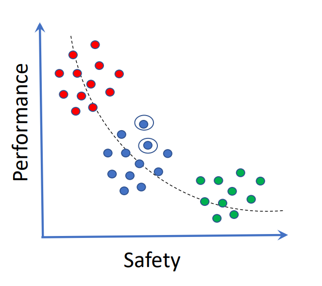
| Figure 5.4.: | Performance-safety tradeoff. Each dot represents a scenario. The optimal scenarios are circled. |
Figure 5.4 shows an example of a performance-safety graph. A rough sketch of what this might entail is as follows: if an intersection has a high performance and no severe events, it is ideal. It is acceptable if an intersection has low performance with no severe events. It is also potentially acceptable with high performance and a few severe events (still avoiding crashes). However, it is unacceptable if an intersection has a low performance and multiple severe events. Thus, using the Pareto curve in the performance-safety graph, a traffic engineer can select a configuration that improves intersection safety without a substantial drop in intersection performance.
Some possible countermeasures are:
We demonstrate the use of the evaluation engine for improving intersection safety in Section 5.4.
This section presents a case study on a representative traffic intersection under different pedestrian and vehicle demand conditions. This case study demonstrates our evaluation engine’s effectiveness in analyzing an intersection’s safety and performance and the impact of any countermeasures in improving the safety of an intersection.
| Table 5.1.: | The details of the intersection used in the case study. The intersection is located in Gainesville, Florida, USA. The column “Speed Limit” gives the major/minor street speed limits. |
ID | Intersection | Speed Limit (mph) | Pedestrian Presence (%) | Left-Turn Type | Flashing Yellow Arrow | Right-Turn on Red |
1 | University Ave. & 17th St. | 25/25 | 41.8 | Protected/ Permissive | Yes | Yes |
Characteristics of the intersection are shown in Table 5.1. Videos from this intersection were collected for a week in November 2021, between 6 AM and 11 PM. Thus, over 100 hours of video footage were collected and processed for the spatiotemporal study. We collected several videos at other times for the evaluation of countermeasures. The high-resolution controller logs were also collected for information about signal phasing during the same period. The speed limit column gives the major/minor street speed limits, while the pedestrian presence column in Table 5.1 provides the percentage presence of pedestrians among all users, pedestrians, and vehicles.
The observations and analyses for the intersection are presented here based on a time-of-day segmentation obtained using the changes in the signal timing patterns. The time segments are defined as follows:
| For weekdays: | |
| AM Peak | 07:00 – 09:30 |
| Off-Peak | 09:30 – 11:00 |
| Midday Peak | 11:00 – 14:30 |
| PM Peak | 14:30 – 18:00 |
This chapter will refer to intersections by ID, and because we are presenting one representative intersection, we will use ID 1. We begin with a detailed image of the intersection, study the pedestrian volume during weekdays, identify potential problem areas and solutions, and evaluate feasible countermeasures. Detailed charts for the intersection representing vehicle volume are omitted for conciseness. Instead, the peak vehicle volume in any one direction is cited as a reference point.
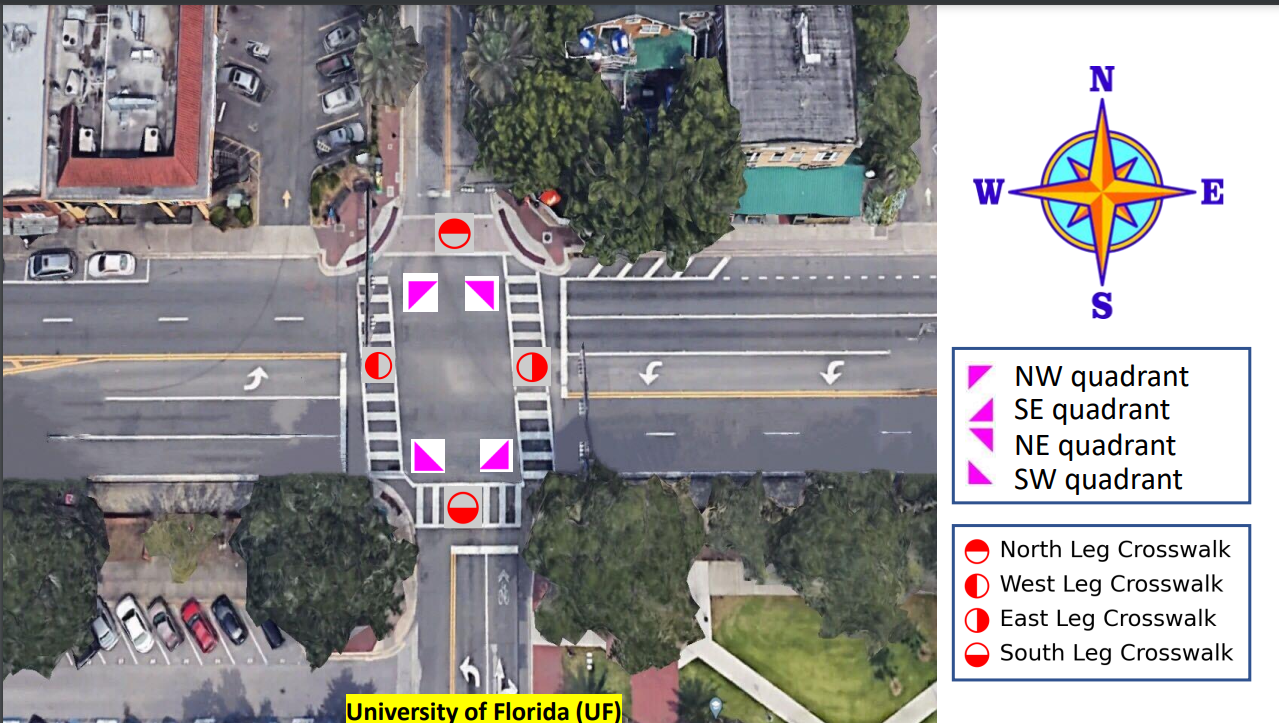
| Figure 5.5.: | Intersection 1: Crosswalks and intersection quadrants are marked. The University of Florida (UF) is at the south of the intersection. University Avenue, the arterial adjacent to UF, runs east to west. The intersection has a heavy pedestrian and vehicle presence. The size of the intersection is quite small, and it serves many pedestrians throughout the day and night and a large number of vehicles. The main issue at this intersection is P2V conflicts. |
Figure 5.5 shows Intersection 1 near the UF. This intersection has a maximum volume of more than 700 vehicles per hour (EBT, PM peak). We start by analyzing the volume and conflict characteristics at this intersection.
Figure 5.6 shows the pedestrian volume during the weekdays. There is increased pedestrian traffic during the midday and PM peaks, coinciding with lunch hour and class dismissal times. Thursday has sparse traffic in the morning for the Veteran’s Day holiday, though the volume picks up later in the day. At its peak, there are about 120 pedestrians per hour using crosswalks. The pedestrian volume is higher on the west crosswalk because more restaurants are accessible across the west leg.
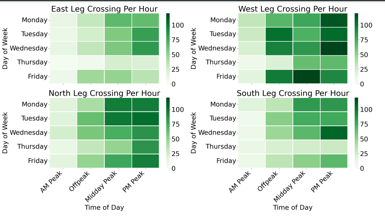
| Figure 5.6.: | Intersection 1: Pedestrian volume during the weekdays. There is an increase during midday and PM peaks, coinciding with lunch hour and class dismissal times. At its peak, there are about 120 pedestrians per hour. The pedestrian volume is higher on the west crosswalk because more restaurants are accessible across the west leg. The gradient color scale on the right displays the number of vehicles. |
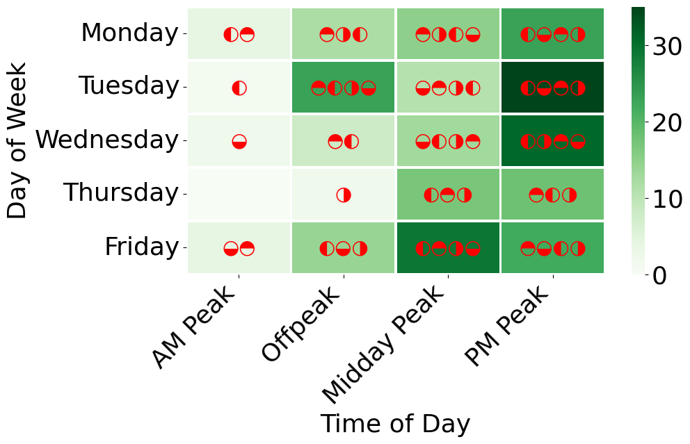
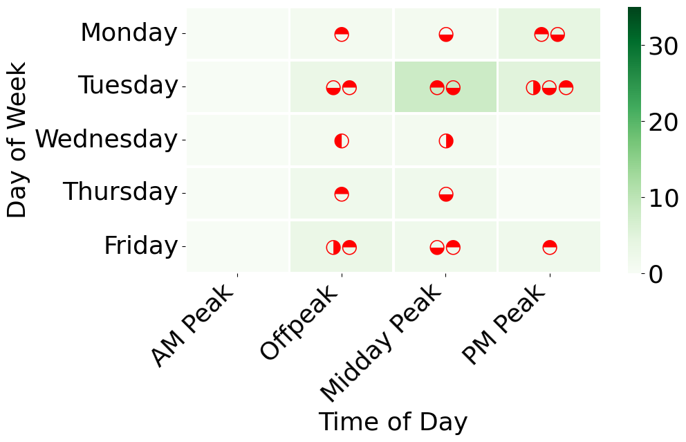
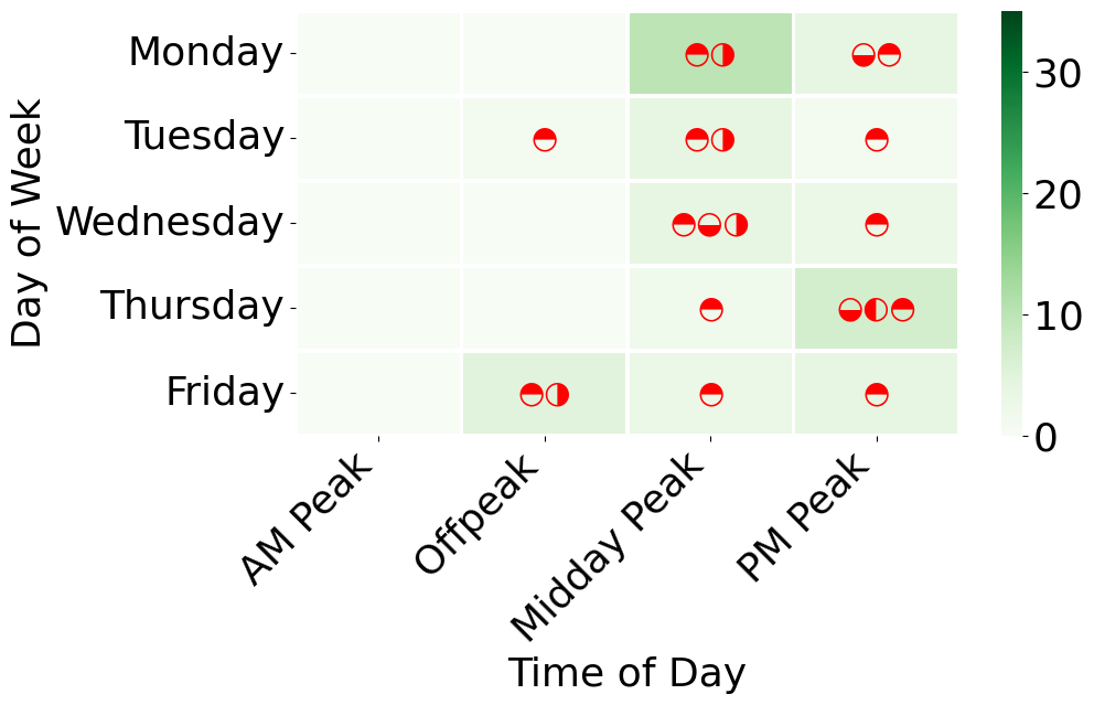
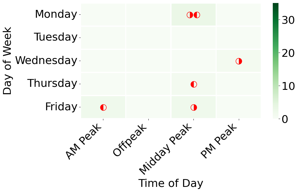
| Figure 5.7.: | Intersection 1: P2V conflicts during the weekdays. Overall, there are many P2V conflicts at this intersection. The gradient color scale on the right displays the conflict count. |
Figure 5.7 shows P2V conflicts during the weekdays. Many conflicts exist on all crosswalk legs, particularly involving left-turning vehicles with pedestrians on the far-side [parallel opposite] crosswalk, as shown in 5.7a. This intersection has protected/permissive left turns. The vehicles often initiate a left turn in the permissive phase, even in the presence of pedestrians on the far-side [parallel opposite] crosswalk. Pedestrians sometimes violate their walk signal and start crossing while a protected left turn is being served.
There were several other conflicts where a right-turning vehicle did not yield to a pedestrian on the adjacent parallel or the near-side crosswalk (Figure 5.7c). The conflicts involving a through-vehicle and a pedestrian (Figure 5.7d) are likely the pedestrian’s fault because vehicles tend to follow their signals at this intersection.
Figure 5.8 shows the V2V conflicts during the weekdays. There are far fewer V2V conflicts compared to P2V conflicts. We can see that the NE quadrant is affected during the AM Peak for RFT conflicts because there is a heavy inflow of people going to work. Both the NE and the SW quadrants are high in LOT conflicts during the PM peak because many cars take EBL and WBL permissive turns, and the uptick in WBT and EBT traffic during the PM peak compounds the problem.
| Figure 5.8.: | Intersection 1: V2V conflicts during the weekdays. There are far fewer V2V conflicts compared to P2V conflicts. The PM peak is particularly affected, most likely due to an outflow of workers from UF. The gradient color scale on the right represents the conflict count. |
The excessively high P2V conflicts at this intersection may be addressed by applying LPI or EPP in the afternoon to address the conflicts in Figures 5.7a and 5.7b. A no-right-turn-on-red directive may reduce the conflicts involving right-turning vehicles in Figure 5.7c.
For the V2V LOT conflicts, split phasing of the major phases at this intersection, especially during the PM peak, might fix this issue, though this will impact performance.
EPP is implemented in this intersection on Thursday, Friday, and Saturday evenings, 8 PM to 1 AM, because the P2V conflicts may be very dangerous at night. Specifically, many bars and nightclubs in the area draw the predominantly young college student population. The evening traffic for one hour, 8–9 PM, was collected and analyzed for Wednesdays (no countermeasure) and Thursdays (with EPP countermeasure). The P2V conflicts are presented in Figures 5.9a and 5.9b, respectively. The benefit of the EPP is clearly seen: most P2V conflicts are resolved in Figure 5.9b. The only conflict (on Thursday, April 21, 2022) happened because the pedestrian violated the walk signal. The pedestrian volume is illustrated in Figures 5.10a and 5.10b for Wednesdays and Thursdays, respectively.
Performance-Safety Tradeoff: The performance is impacted while the EPP effectively resolves P2V conflicts. To evaluate the approximate impact on the performance of the intersection, we measured the volume of vehicles on both days and find fewer vehicles per 10-minute intervals with EPP implemented (Figures 5.10a and 5.10b). However, the decrease in volume was not particularly large. This indicates that the performance cost of the countermeasure is minimal. Therefore, the added safety of the exclusive pedestrian phase is well worth the slight inconvenience to the vehicles. Figure 5.11 aggregated the P2V conflicts and vehicle volume on Wednesdays when there were no countermeasures to Thursdays when the EPP countermeasure was in effect.
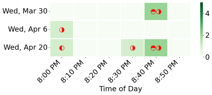
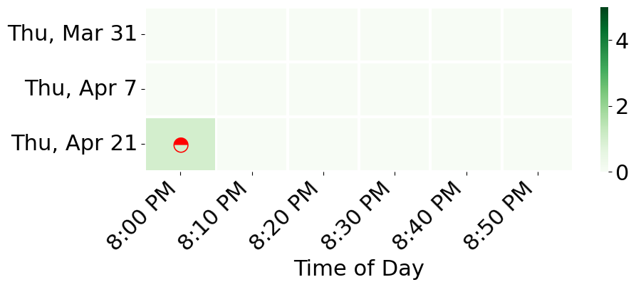
| Figure 5.9.: | Intersection 1: Countermeasure EPP. From 8 PM onward, EPP is implemented on Thursday, Friday, and Saturday. The heatmap on the left shows the P2V conflict distribution on Wednesdays and compares that with the countermeasure implemented on Thursdays. The reduction in the number of conflicts is pronounced. The one conflict on April 21 was due to a pedestrian violating signals. The gradient color scale represents the conflict count. |
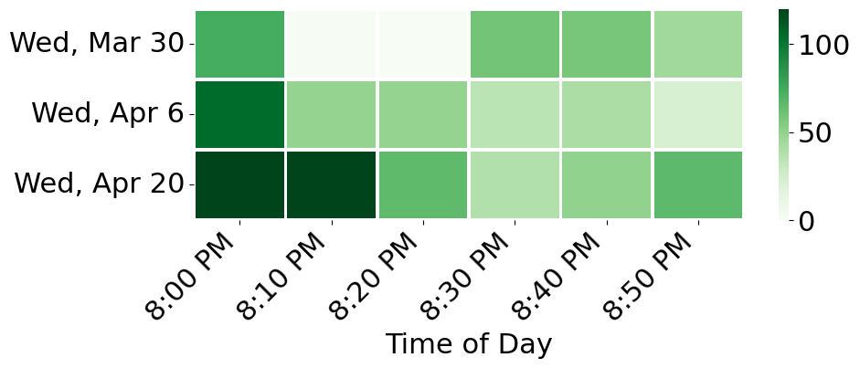
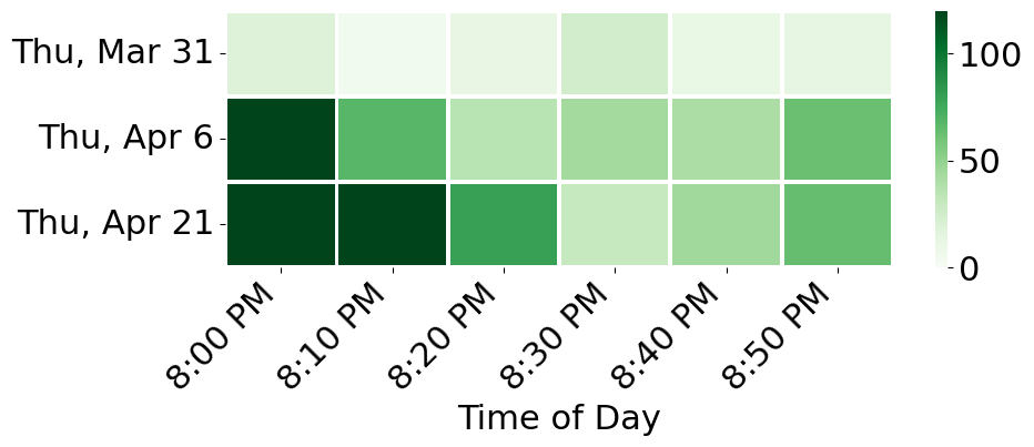
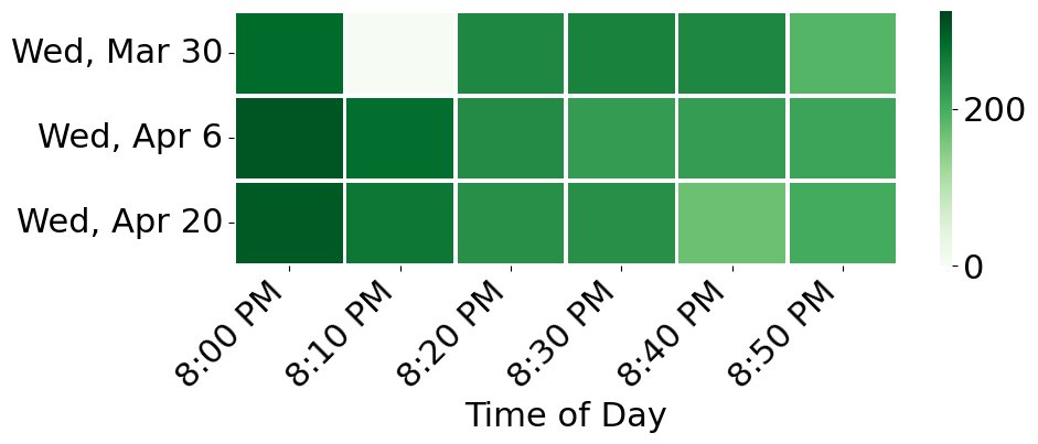
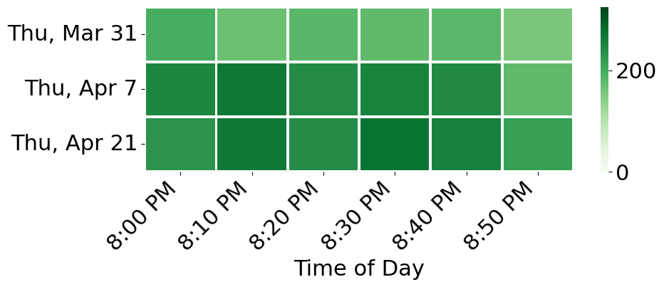
| Figure 5.10.: | Intersection 1: Pedestrian and vehicle volume during the countermeasure study period. On Wednesday, March 30, between 8:10 and 8:20 PM, the video collected was corrupted; hence, it was dropped from the analysis. The gradient color scale represents the vehicle count. |
| Figure 5.11.: | Comparison of the number of P2V conflicts on the case study intersection on Wednesday evening when EPP is not implemented and Thursday evening when EPP is implemented. Note the significant decrease in conflicts at a similar volume of traffic. |
| Conflicts | Vehicle Volumes | ||
Wednesdays | Thursdays | Wednesdays | Thursdays |
7 | 1 | 4355 | 4002 |
Road safety is highly relevant in today’s societies, as vehicle collisions claim lives every day. Intersections especially are prone to crashes which lead to the worst outcomes. Recent rapid improvements in video collection and processing technologies enable us to identify and alleviate dangerous situations. Conflict and volume hotspots are detected, and intersection performance is analyzed using trajectory data, severe events, and signal phasing. This chapter’s extensive analysis and discussion of a representative intersection demonstrate the selection of appropriate countermeasures. Additionally, we evaluate the efficacy of countermeasures in an understandable and replicable manner.
Our evaluation engine takes inputs from the intersection: trajectory, severe event, and signal phasing data. The inputs are generated using our previous work on processing intersection videos [90] and from the intersection ATC. The evaluation engine has three primary modules: the first computes pedestrian and vehicle volume hotspots; the second calculates pedestrian-vehicle (P2V) and vehicle-vehicle (V2V) conflict hotspots; the third evaluates intersection service as a proxy to intersection performance for the study period. The evaluation engine then outputs histograms and conflict and volume hotspot charts, where each conflict chart is annotated with information that identifies the traffic phases involved in the conflicts. These outputs allow for possible use by researchers and traffic engineers. We also demonstrate how to compute performance-safety tradeoff charts. The knowledge about performance-safety tradeoffs is crucial for arriving at effective countermeasures with minimal impact on intersection performance. The readability of the tradeoff graph makes it easy to compare and select appropriate countermeasures. We demonstrate the operation of the evaluation engine on a busy intersection—“Intersection 1”—adjacent to a university campus, using more than a week of data. More than 100 hours of video were collected and processed in the demonstration of our engine, and with the level of automation achieved, more videos can be analyzed at little cost.
Intersection 1 is located near UF and has a high pedestrian presence. The intersection has a maximum vehicle volume of more than 700 vehicles per hour during the PM peak. The number of pedestrians on the west leg is consistently the largest because of local restaurants, reflected in the more significant number of P2V conflicts with pedestrians on the west leg. The number of V2V conflicts is relatively small and is primarily associated with people coming to and going from work. A large number of P2V conflicts and the inherent danger due to evening conflicts influence the implementation of an EPP countermeasure. The countermeasure decreases the number of P2V conflicts a great deal. Furthermore, the impact on performance is insignificant relative to the safety enhancement at the intersection, justifying the continued use of the countermeasure.
This chapter aims to help the practitioner find any safety issues within an intersection that may not have resulted in a crash but could result in one in the future. This work results from a close interactive feedback loop between researchers and traffic practitioners. For example, our analysis uncovered the everyday pedestrian-vehicle conflict situations observed in Intersection 1, where the pedestrian was given a walk signal, and the left-turning vehicles were shown a permissive left a few seconds later. The conflicts did not lead to crashes or injuries but often to near-miss conflicts. This information finally allowed the practitioners to test the countermeasure of exclusive pedestrian signaling in Intersection 1. As a result of implementing the exclusive pedestrian phases, vehicles are stopped on all legs, and pedestrians may cross in any direction. This made the intersection safer for pedestrians.
A direction of potential future study is the automation of additional steps in the process we have outlined, including, but not limited to, the suggestion, analysis, and implementation of countermeasures on the fly. Also, the precept of a performance-safety tradeoff in intersection analysis developed here can be applied further and potentially more broadly in road safety.
Road intersections show complex geometry and traffic rules and require drivers’ timely maneuvers. The Federal Highway Administration (FHWA) has reported that more than 50% of fatal and injury-causing crashes occur at or near intersections. Of all the intersection-related crashes, only about 4% are caused by vehicle or environmental reasons, and 96% are attributed to drivers [129]. Factors contributing to driver-attributed crashes at intersections include inadequate surveillance, false assumptions regarding other drivers’ actions, obstructed views, illegal maneuvers, internal distractions, and misjudgments of gaps, speed, etc. [129]. Potential solutions for reducing crashes focus on providing driver assistance in controlling the vehicle or giving timely warnings of potential risks. To this end, predictive algorithms are proposed. For example, by tracking the surrounding vehicles, one can estimate their intended maneuvers, predict their future motion, and estimate the risk of collision. Previous studies [130, 131, 132, 133] have focused on the automated vehicle (AV) and advanced driver assistance system (ADAS) solutions. These approaches rely on onboard sensors like LiDAR, radar, and vision sensors. However, the onboard sensors have limitations, such as limited detection range or field of view, low resolution, drifting position estimation, and sensor imprecision. Therefore, we propose incorporating assistance from existing and planned intersection video infrastructure to improve safety. An essential basis of the information such systems will provide is real-time knowledge of the motions of other vehicles in the intersection and their potential to collide with other vehicles, i.e., trajectory prediction.
In this chapter, we tackle the problem of robust and flexible vehicle trajectory prediction at intersections from surveillance videos, aiming to give early warnings to vehicles about possible collisions and abnormal behaviors. Our proposed approach only requires vision sensors – no signal data are needed—and can be applied to signalized and unsignalized intersections. Our approach requires a setup stage, namely, (i) Google Maps alignment, (ii) learning typical motion patterns from historical data, and (iii) training the trajectory prediction model. After the setup, our model can make real-time predictions of all the vehicles’ trajectories within the intersection. We also consider the noise the automatic vehicle tracking algorithms introduced and the varying lengths of trajectories captured.
The main contributions of the chapter are as follows:
The rest of this chapter is organized as follows. Section 6.2 presents the related works on trajectory prediction methods. Section 6.3 gives an overview of our proposed approach, consisting of offline learning and online prediction phases. Section 6.4 describes the methodology of offline trajectory clustering and prototype generation. Section 6.5 presents the CCS transformations and the trajectory prediction model. Section 6.6 reports our experimental settings and quantitative and qualitative results. We conclude with a few observations in Section 6.7.
Vehicle motion or trajectory prediction has been studied extensively over the last two decades and is mainly used in ADAS and AV. The work in Lef�vre et al. [134] organized motion prediction approaches into three categories: physics-based, maneuver-based, and interaction-aware. Our approach falls into the maneuver-based category. The work in [134] further divides the maneuver-based approaches into prototype-based and intention estimation. Our approach can be classified as prototype-based.
Prototype-based approaches assume that vehicle motion can be grouped into a finite set of clusters. A prototype trajectory is learned for each cluster as its representative. In the case of four-way intersections, there are mainly twelve motion patterns, namely left turn, right turn, and going straight from the four directions. For road sections, typical motion patterns are lane keeping, lane change to the left, and lane change to the right. An early work [135] adopts a statistical approach where the mean and standard deviation represent clusters of motion patterns. Later works [136, 137, 138] represent motion patterns with Gaussian processes (GP) due to their ability to capture spatiotemporal characteristics of traffic situations. One drawback of GP models lies in their computational complexity. As a nonparametric approach, the number of parameters grows as more training samples are provided. In a surveillance setting, a nonparametric approach will be slow and expensive to leverage the vast amount of data captured from cameras. In this work, our proposed approach fits a compact model to the training data and incorporates the prototype trajectories to make more informed predictions.
Trajectories are sequences of locations, velocities, etc. Recurrent neural networks (RNNs), especially long short-term memory (LSTM) and gated recurrent units (GRUs), have been explored and broadly evaluated for the task of sequence generation and prediction. Over the last five years, RNN and its variants have been gaining popularity in trajectory prediction. The work in Alahi et al. [139] first applied an LSTM model to learn general human motions and predict their future trajectories. Later works [140, 141, 142, 143] extended the idea to vehicle trajectory predictions, enabling vehicles to reason about the future motion of other surrounding vehicles. To the best of our knowledge, no work utilizes a deep learning-based trajectory prediction model from surveillance vision systems. Unlike the above approaches for autonomous vehicles or ADAS, where modeling interaction is essential, our approach will be applied to give early warnings to vehicles entering intersections; hence, we focus on typical motion pattern finding and efficient online functioning.
The chapter is divided into two main components: an offline phase in which trajectories are clustered and promising prototypes are found. This is followed by an online step in which different LSTMs are constructed for trajectory prediction. The second phase necessarily uses the prototype information from the first phase. In this section, we give a procedural description of our algorithm workflow. Figure 6.1 concisely summarizes the workflow.
The offline phase can be performed periodically to capture the dynamics of traffic evolution (e.g., road construction that causes vehicle detour) or done once for setup if the intersection geometry remains unchanged. There are two main tasks in the offline phase: (i) finding common motion patterns and their representatives and (ii) training the LSTM-ED (long short-term memory encoder-decoder) trajectory prediction model.
The trajectories are captured by a vision-based tracking algorithm and are stored in the database. We refer to the trajectories in the database as historical trajectories. We use a portion of historical trajectories to learn common motion patterns using a coarse-to-fine clustering algorithm and find prototypes to represent each motion cluster. A filtering and smoothing algorithm is applied before clustering to generate longer and smoother prototype trajectories. Lastly, the trajectory prediction model to be used in the online phase is trained in the offline phase.
The online phase receives real-time captured trajectories from the online tracking algorithm. We first detect whether the vehicle is waiting for traffic signals using the stay point detection algorithm from Cai et al. [144]. We start making predictions when the vehicle starts moving. We match a partial trajectory from a moving vehicle with prototype trajectories from the offline phase based on distance measurements. We then feed the partial trajectory, matching prototypes, and duration to be predicted into the trajectory prediction model to output its future trajectory.
This section introduces the methods used to cluster trajectories and find prototypes.
Vehicles at an intersection exhibit common motion patterns, and their trajectories can be grouped into clusters. One or more finer clusters can be found within each cluster of the same moving direction, as there might be multiple entering and exiting lanes of the same motion. Our clustering approach is, therefore, a two-step process where we first cluster the trajectories based on their direction of motion and next cluster the trajectories for a given motion using spectral clustering. In this section, we describe the clustering based on motion direction, followed by the description of a new distance measure for spectral clustering. Finally, we describe our spectral clustering approach.
When we analyze a collection of trajectories, one of the first steps is automatically identifying the trajectory phase. As shown in Figure 6.2, the vehicle phase system assigns a single number for both through and right-turn movements. We find it helpful first to have a separate category for the right-turn vehicular movement. So, in addition to the eight bins, each storing trajectories of a particular phase, we append four more bins for storing the trajectories making right turns for phases 2, 4, 6, and 8.
The motion direction of a trajectory can be represented as the vector connecting the start and end points. This process was explained in detail in Chapter 3.
After partitioning the trajectories by motion direction into bins, we apply spectral clustering to the trajectories of each bin. We used a new distance measure for computing the distance between two trajectories in the same bin. This is described next.
Spectral clustering is applied next to the trajectories in the same direction bins, and we get clusters of trajectories with the same movement. Spectral clustering may also be used to identify outliers or anomalous trajectories that are not similar to any other trajectories in the same bin. The details of our spectral clustering implementation may be found in Banerjee et al. [145].
From our clustering algorithm, clusters of motion patterns are found. This section presents our approach to generating prototype trajectories for each cluster.
Many trajectories extracted from the traffic video are incomplete, meaning they either appear from the middle of the intersection or disappear within it. These trajectories are as helpful as complete ones in the LSTM-ED model training. However, we prefer complete trajectories for prototype generation for two reasons: (1) complete trajectories are spatially aligned because they start and end in the same regions, and (2) the distance measure we use performs better with a longer reference trajectory.
Trajectories that start at an intersection entrance and end at an intersection exit are considered complete. We annotate the intersection boundary as a polygon. For each motion pattern, we annotate its enter line and exit line. We consider a trajectory complete only when its starting point is close to the entering line, and its ending point is close to the exit line. The left part of Figure 6.3 shows the complete trajectories from one cluster.
Given a set of complete trajectories from a cluster, we aim to find a representative for the cluster by averaging the trajectories. We represent the complete trajectories as 2-D cubic splines, denoted as S, where x and y coordinates of a trajectory are parameterized by t:
 | (6.1) |
where t’s are equally-spaced break points in the range of �0;1�. As the complete trajectories are roughly spatially aligned, an average trajectory for each cluster can be found by
 | (6.2) |
where Sj is a complete trajectory from the given set from cluster c, and mc is the number of trajectories. After obtaining the average trajectories, the last step is to reparametrize and re-scale the splines. We adopt the arc-length parameterization algorithm from [146], which results in equally spaced control points. We then re-scale the splines so that consecutive points of a spline have a distance of one meter. Figure 6.4 shows the prototypes we obtained for an intersection.
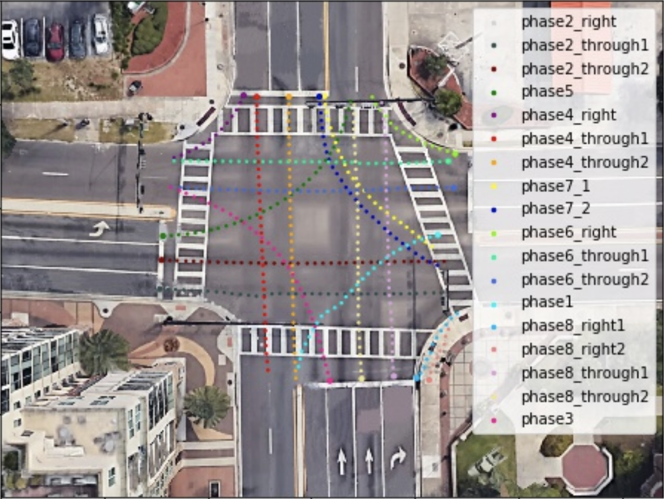
| Figure 6.4.: | The resulting prototypes. Note that the slight deviation of some prototypes is caused by imperfect Google Map alignment. |
In this section, we present our trajectory prediction model. A summary of the approach follows. The trajectories represented initially in cartesian coordinates are first transformed to CCS. These CCS trajectories are then fed to the LSTM-ED model for training and inference. In the following three sections, we define the trajectory prediction problem in section 6.5.1, introduce the CCS and transformations from and to cartesian coordinates in section 6.5.2, and describe the architecture, training, and inference using LSTM-ED in section 6.5.3.
Given an observed partial trajectory of the i-th vehicle in CCS:
 | (6.3) |
the model predicts the future trajectory:
 | (6.4) |
where tobs is the current time step of the trajectory measured in one-second intervals and tobs � tpred is the final time step of the predicted trajectory.
Curvilinear coordinate systems (CCSs) are a natural fit for our problem of trajectory prediction. Consider the problem of predicting left-turn trajectories at intersections. In standard Euclidean coordinates, the velocity vector changes its orientation continuously through the turn, whereas a reparameterization of the velocity along the curve has the advantage of better inertia representation. CCSs are also akin to using Lagrangian frames in fluid mechanics (or the viewpoint from the boat in a river) as opposed to the Eulerian frame (or the viewpoint from the riverbank watching the boat float by). The work in [147] uses curvilinear coordinates to impose roadway geometry constraints to motion tracking and behavior reasoning algorithms. We extend the idea to intersection geometry, which implicitly constrains the vehicle trajectories to standard trajectory templates. We propose to use the CCS, defined as the shape of a prototype trajectory. Partial trajectories matching the prototype are assumed to move along with it, with an offset. The prediction is largely simplified in the CCS because the model only needs to learn the difference between a new trajectory and the average historical trajectories conforming to the same motion pattern.
For a vehicle entering an intersection, the possible motion patterns can be found by matching with trajectory prototypes. Most motion patterns can be ruled out, as their distances to the query trajectory are too far to be considered potential matches. In this work, we only consider the closest two prototype trajectories. Each prototype trajectory defines a curvilinear coordinate system with s and n axes—essentially the tangent and normal at each point along the curve. The s-axis is defined along the shape of a prototype, with arc length coordinates used, while the n-axis is defined to be perpendicular to the s-axis at every point on the curve, giving us a measure of how far a point is from the curve, as shown in Figure 6.5. In the rest of this section, we describe the transformations between the image coordinate system (ICS) and the CCS, where image coordinates (IC) refer to Google Maps-aligned intersection image coordinates. We denote a point in IC as �xp;yp�, and its corresponding point in CC as �sp;np�, as shown in Figure 6.5.
Our prototype trajectories are sampled from continuous splines, as in section 6.4.2, and determining the closest point on a spline from a query point requires using optimization methods. These are now described. Given p with coordinates xp;yp in the ICS, we aim to find the CCS’s corresponding sp;np. We first find sp by finding the closest point on spline S to the point p, which can be formulated as the following minimization problem:
 | (6.5) |
We use a standard limited-memory optimization algorithm (BFGS; available in Python scientific libraries) to solve for sp. Once sp is determined, we turn our attention to np. First, jnpj is defined as the distance between p and p0. The sign of np is determined by:
 | (6.6) |
where sgn is the sign of a number, � is the cross product, q0 is a point near p0 with a slightly smaller s-value and � denotes a small number. Vector q0p0 estimates the growing direction of S at point p0. So far, we have given the procedure of transforming from ICS to CCS. We now examine the opposite direction.
Given sp;np in the CCS, we aim to find the corresponding xp;yp in the ICS. This is a relatively easy process because the transformation has a convenient closed-form expression:
 | (6.7) |
where e? is the unit vector perpendicular to S at point p0, which can be found from the derivative of S. In summary, the use of CCS simplifies the task for trajectory prediction because it decouples the two coordinates to some extent. The S-coordinate mainly captures the speed along the road while the N-coordinate mainly captures the speed off the road (e.g. lane changes or abnormal behavior). The coupling of prototype trajectories to a “Lagrangian” coordinate system is a vital contribution of this work.
LSTM networks are designed and proven effective for sequence modeling and prediction tasks. Thus, they are well-suited for trajectories represented as a sequence of coordinates. We adopt the encoder-decoder architecture to cope with variable lengths of trajectories and prediction periods. The encoder encodes observed partial trajectories to a fixed-length internal representation, and the decoder decodes the state and predicts possible future motions for a given period. Besides the internal vector from the encoder, cluster belonging is also provided as input to the decoder. In this way, the decoder learns to predict differently considering its cluster.
The encoder and decoder have two layers: fully connected (FC) and LSTM layers. The FC layer is an embedding function that embeds locations into a fixed-length vector. The embedding will then be fed to the LSTM layer. The encoder encodes the observed trajectory into the LSTM’s last hidden state hi�tobs�. The decoder takes hi�tobs� concatenated with the one-hot-encoded cluster class vector as input and is trained to generate its future trajectory Yi.
We adopt the L2 loss for training, which measures the distance between the predicted and the ground-truth trajectories. As vehicles pass an intersection at different speeds, the number of trajectory points captured in the intersection varies over a wide range. For example, a left turn trajectory usually has more trajectory points captured than a straight heading trajectory because a left turn vehicle will slow down as it enters the intersection. In contrast, a straight heading vehicle tends to be at the maximum speed limit. For this reason, we enable the model to encode variable-length observations and decode variable-length predictions. We achieve this by splitting a training sample into an observation and prediction sequence with a random ratio tobs:tpred so that the model is trained from mixed-length data and will learn to make variable-length predictions.
At inference time, the cluster class of a trajectory i is unknown. The model first infers cluster class by matching with all prototype trajectories. The degree of belonging of trajectory tri to cluster class C�m� is calculated by inverse distance weighting:
 | (6.8) |
where d is the distance measure introduced in section 3.5.1, and trC�j� represents the prototype trajectory of class C�j�. If the trajectory has a similar degree of belonging to M classes, the model will output M predictions. For each possible cluster class, the model will make the corresponding prediction. To be more specific, for each possible C�j�, the corresponding representation in CCS as well as the one-hot cluster vector, will be fed to the LSTM-ED model, which then makes its future prediction with ”probability” uC�j��tri�. We set M to 2 based on intersection geometry because each lane of an intersection usually allows two or fewer motion patterns (e.g., heading straight and right turn).
The embedding dimension is set to 64 for both the encoder and decoder. The encoder’s LSTM layer has a hidden state of dimension 64, and the decoder’s LSTM layer has a hidden state of dimension 64 + nc. We use the Adam optimizer with a 1 � 10�4 learning rate. The tobs:tpred ratio is randomly chosen in the range �0:3;0:7�.
We evaluated the proposed approaches on the collected trajectory dataset from surveillance fisheye cameras at three intersections. Section 6.6.1 describes our data collection methods and preprocessing steps to obtain Google Maps-aligned trajectories. Section 6.6.2 compared our trajectory prediction model with baseline methods. Finally, Section 6.6.3 evaluates the trajectory prediction pipeline for variable-length observation and prediction period.
Our intersection trajectory dataset is obtained from three busy intersections in Gainesville, Florida. The surveillance cameras have a circular fisheye lens and a 10-fps frame rate. From our previous work [68], we have the mapping from fisheye video pixels to Google Maps locations. A detection and tracking pipeline is running periodically to automate the trajectory capture process. We clean the dataset using rule-based filtering. We impose speed limits within the intersection and non-self-intersecting constraints on trajectories. We also applied a trajectory smoothing algorithm to compensate for detection imprecision. In addition, as the traffic signal phase is unknown in our setting, we exclude the stay points of trajectories before entering the intersection. After the above process, we obtain roughly 15,000 trajectories for each intersection, split into training, validation, and testing sets with a roughly 7:1:2 ratio. The validation set is used in LSTM-ED training to avoid overfitting. We refer to the three intersections simply as Intersection 1, Intersection 2, and Intersection 3.
In this section, we evaluate the performance of the proposed trajectory prediction model and compare it with baseline models. This experiment is performed on Intersection 1, and we assume the ground-truth cluster class of each trajectory is known. We compare the proposed model (LSTM-ED CCS) with two baseline models:
We adopt the following two metrics for prediction evaluation:
We show the prediction errors of different observation and prediction periods. We set a threshold for minimum trajectory length for evaluation to ensure fair comparison for different period settings. Only trajectories with more than 40 timestamps are chosen because the maximum of observation and prediction timestamps is 40, as shown in Table 6.1. In this way, the same set of trajectories is used for each setting instead of some trajectories (less than 40 timestamps) only used in shorter-period settings. Thus, the experimental result truly reflects the model’s performance for different observation and prediction periods. The prediction errors are reported in Table 6.1.
| Table 6.1.: | Comparison of trajectory prediction approaches given ground-truth cluster class |
| Observation Length | 10 | 20 | 30 | ||||||
| Prediction Length | 10 | 20 | 30 | 10 | 20 | 10 | |||
| ADE | 0.75 | 1.86 | 2.76 | 0.45 | 1.20 | 0.35 | ||
| FDE | 2.76 | 4.96 | 6.08 | 2.34 | 4.58 | 2.69 | |||
| ADE | 0.61 | 1.24 | 1.96 | 0.47 | 0.91 | 0.45 | ||
| FDE | 1.13 | 2.51 | 4.17 | 0.86 | 1.97 | 0.84 | |||
| ADE | 0.51 | 1.10 | 1.76 | 0.45 | 0.91 | 0.47 | ||
| FDE | 0.97 | 2.32 | 3.61 | 0.81 | 1.87 | 0.87 | |||
LSTM-ED CCS outperforms the two baseline models in almost every setting. GP tends to have a large FDE, and the prediction result also looks unsmooth. LSTM-ED ICS performs similarly on shorter prediction periods as LSTM-ED CCS but worse on more extended prediction periods.
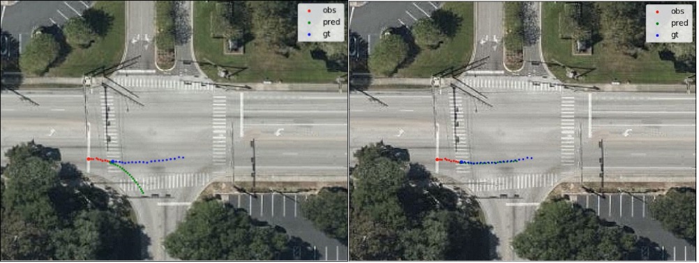
| Figure 6.7.: | Two predictions at inference time. The red, blue, and green points represent observed, ground-truth future, and predicted points of a trajectory, respectively. |
Our pipeline consists of cluster class determination and trajectory prediction. In other words, unlike the previous experiment, the ground-truth cluster class is unknown to the LSTM-ED model. We evaluated the pipeline at all three intersections. The quantitative result is reported in Table 6.2. The qualitative result is shown in Figure 6.8. As explained in section 6.5.3, our model produces multiple outputs if the observed trajectory matches with numerous prototypes. Figure 6.7 shows one example of multiple outputs. From the observed trajectory, going straight and right turn are both likely.
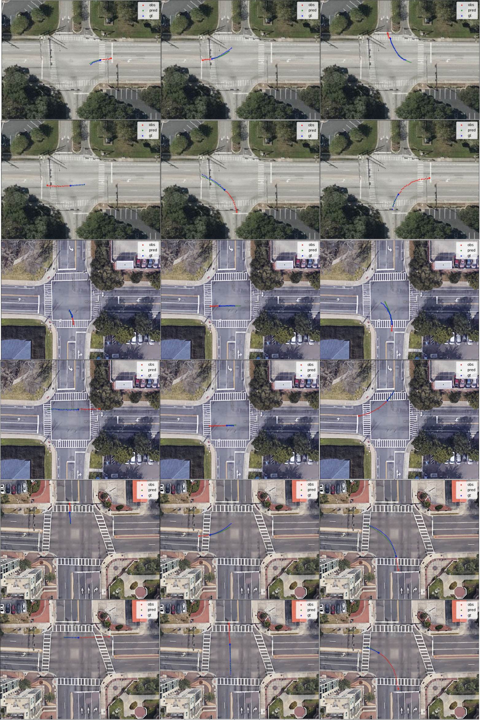
| Figure 6.8.: | Samples of the prediction results on Intersections 1, 2, and 3 (top to bottom, respectively). |
| Table 6.2.: | Prediction errors for Intersections 1, 2, and 3 |
| Observation Length | 10 | 20 | 30 | |||||
| Prediction Length | 10 | 20 | 30 | 10 | 20 | 10 | ||
| ADE | 0.54 | 1.21 | 2.09 | 0.52 | 1.16 | 0.61 | |
| FDE | 1.02 | 2.70 | 4.83 | 0.97 | 2.61 | 1.15 | ||
| ADE | 0.54 | 1.23 | 2.05 | 0.46 | 0.91 | 0.49 | |
| FDE | 1.03 | 2.72 | 4.29 | 0.79 | 1.90 | 0.82 | ||
| ADE | 0.66 | 1.40 | 2.19 | 0.58 | 1.18 | 0.54 | |
| FDE | 1.24 | 2.89 | 4.38 | 1.03 | 2.44 | 0.99 | ||
A real-time trajectory prediction approach coupled with aligned Google Maps information is proposed in this chapter. Our approach uses a historical trajectory database and finds typical motion patterns to guide future prediction. Given this prior information, our approach can make reasonable predictions based on variable starting position, observation period, and prediction period. Experimental results on three intersections show the effectiveness and extensibility of our approach. In the immediate future, we plan to integrate our trajectory prediction module into an early warning system. We believe our work will help increase intersection safety.
Mitigating traffic congestion and improving safety are the essential cornerstones of transportation for smart cities. With growing urbanization worldwide, traffic congestion along high-volume signalized traffic corridors (arterials) is a significant concern. Congestion negatively affects productivity, leading to loss of work hours, thus impacting the economy. Congestion also impacts the well-being of society and the environment [4, 148].
One of the critical congestion measures is arterial travel time [149]. This value is a vehicle’s expected travel time to complete its journey along a signalized traffic corridor. It is affected by many factors, such as traffic conditions and departure time. This quantity is easy to interpret by traffic engineers, city authorities, and the general public. Traffic engineers can use travel time to identify problematic locations and timing problems that can improve the overall performance of a traffic system [150, 151, 152, 153, 154, 155]. Current performance evaluations only include a limited comparison of before-and-after travel time data to demonstrate the effectiveness of signal retiming[156] efforts.
Most existing research on travel time estimation focuses on using non-vision sensors such as GPS [157, 158] and loop detectors [159]. Due to the simplicity of implementation and low computational cost, travel time estimation methods based on historical data have been widely used in practice [160, 161]. Other approaches rely on machine learning and data mining of toll collection information [162], probe car [163], highways [164], and trip datasets [165].
However, traffic patterns vary dynamically during the day and globally within the network. There is a need for continuous monitoring and evaluation of signal timing parameters based on performance and fluctuation demands. Travel times have to be calculated at regular intervals. In addition, it is essential to understand the distribution of travel times rather than average travel times because the tail of the distribution gives traffic engineers rich information. Actual travel time often has a multimodal distribution, and the average values are not always sufficient. The advent of video cameras at traffic intersections has opened the possibility of using them for instantaneous travel time computation and is the focus of this chapter.
The novelty of our travel time estimation is twofold. First, we use car signatures to estimate vehicle departure and arrival time from video across multiple cameras. In addition, we leverage signal data in this system obtained from ATSPM logs from the controller. To our best knowledge, this represents the first end-to-end framework that estimates vehicle travel time on corridor intersections using multiple video and signal data.
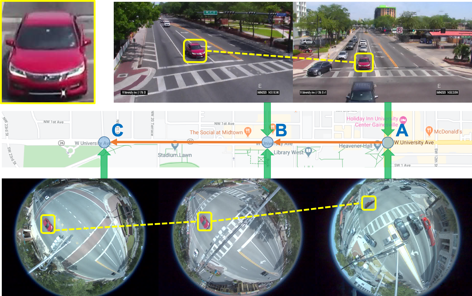
| Figure 7.1.: | An illustration of multi-camera vehicle tracking and travel time estimation problem. In this example, we have three intersections, A, B, and C, in a corridor. They all have one fisheye camera, and A and B have another pan camera. The multi-camera vehicle tracking and travel time estimation problem determine (1) whether the red car is the same vehicle among these intersections and (2) what its arrival and departure times are at each intersection. |
We achieve the above goals by accurately tracking a small subset of vehicles on a corridor or network. Along with reasonably synchronized clocks at each intersection, this will allow for accurate travel time computation for that subset of cars and can be used for travel time computation in general. The latter is a relatively straightforward computation if tracking can be accurately achieved. It is worth noting that it is more critical for the tracking to be accurate for a subset of cars rather than tracking a larger fraction of vehicles with less accuracy. That is because precise tracking can provide good input for re-identifying cars across multiple cameras and thus compute more accurate travel time.
We develop a unified system to track vehicles across multiple video cameras on corridor intersections. It uses a robust signature matching algorithm to handle the variance of vehicle pose under different camera perspectives. This algorithm can efficiently identify signatures of vehicles in real-time and further help the computation of accurate detection of arrival and departure times at each intersection. Some vehicles may have to wait when the light turns red at any signal. This, in general, creates additional delays for a subset of vehicles. Our approach can robustly tackle these challenges.
Additionally, our approach leverages the fact that ordering vehicles from one intersection to another remains relatively the same. This is optional for our approach to be practical, but this property can reduce the computation time requirements for the matching algorithm. Although much of the chapter is described in terms of computing travel times on a corridor, the basic ideas are promising in the extension to work on a mesh of intersections.
In summary, we propose a real-time video processing system for multi-camera vehicle tracking and travel time estimation with the following key contributions:
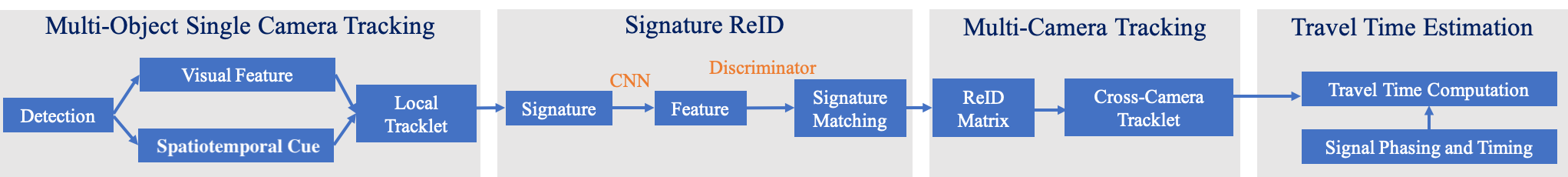
| Figure 7.2.: | An illustration of the pipeline for the proposed method. Given intersection videos as input, a single-camera tracker first detects vehicles and generates local tracklets. Then a ReID discriminator computes matching among vehicles under the constraints of phase information. Finally, we apply a merging algorithm to update tracking results for multi-camera tracking and compute the travel time of each vehicle using the timestamp information. |
Multi-object multi-camera tracking intends to detect and track multiple objects within one camera (tracklets) and then perform multi-camera tracklet matching to derive trajectories of vehicles. The arrival and departure timestamps of the vehicles are then utilized to estimate travel time distribution. The inputs of our method are traffic video data collected from multiple intersections. For the sake of simplicity, we assume a three-camera system with one camera for each of the three successive intersections (corridor intersections). It is easy to generalize these ideas to a more significant number of intersections (e.g., mesh intersections). Each intersection can have one or more cameras, potentially of different types. In particular, the corridor that we experimented with has three intersections, labeled A, B, and C. A and B have one fisheye camera and one pan camera, while C only has one fisheye camera. Thus, this corridor corresponds to two tracking channels: (1) in the fisheye channel, the inputs are video sequences from three fisheye cameras, and (2) in the pan channel, the inputs are video sequences from two pan cameras.
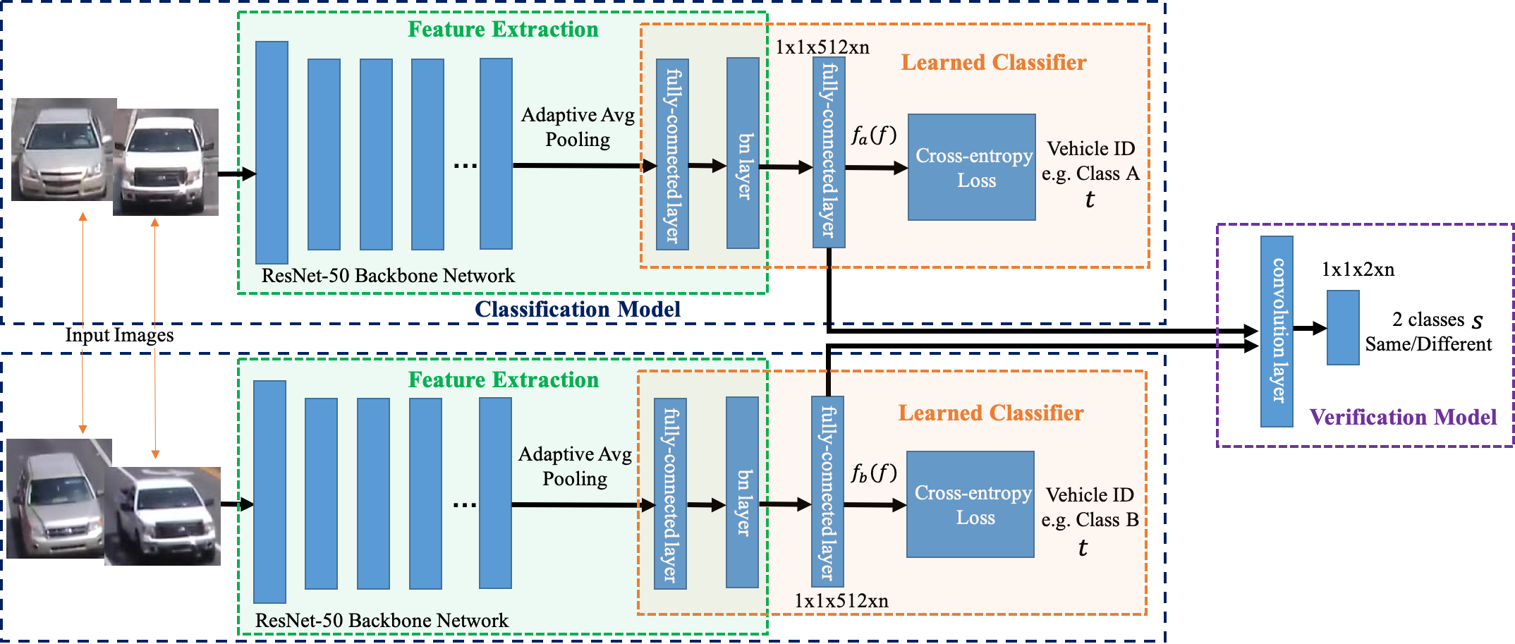
| Figure 7.3.: | An illustration of the network architecture of our proposed two-loss signature ReID model using ResNet-50 as the backbone. |
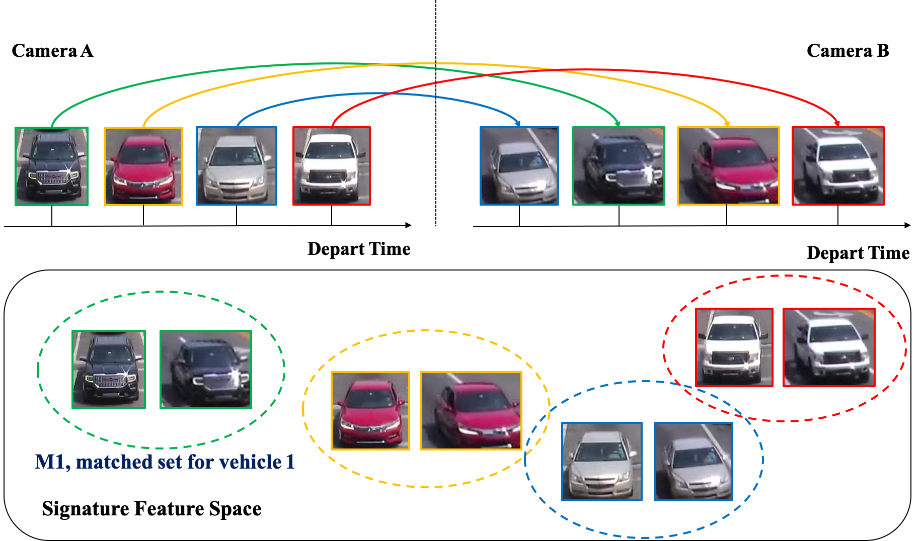
| Figure 7.4.: | An illustration of matched-vehicle sets and their distributions in the feature space. The solid color arrows indicate the one-to-one mapping results. |
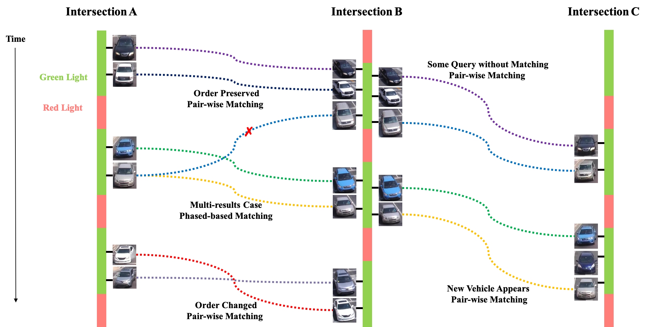
| Figure 7.5.: | An illustration of across-camera matching. Our primary matching strategy is pairwise matching using our discriminator. For cases with multiple matching results, phase information is used as an additional constraint to refine matching. We defined five types of matching cases: (1) order preserved (pairwise matching), where the order of signature sequence does not change among intersections; (2) multi-results case (phased-based matching); (3) order changed (pairwise matching); (4) some query without matching (pairwise matching); and (5) new vehicle appears (pairwise matching). |
Our proposed method contains four major modules, as shown in Figure 7.2:
Additionally, before utilizing the second video-based signature ReID module, we can filter out tracklets using trajectory direction detection (go-straight, turn-left, or turn-right) and only focus on one direction (e.g., traffic flow go-straight from camera A to camera B then camera C).
Each of these modules is described in detail in the following subsections.
We use a deep learning model to detect and track road objects, calculate the speed after deformation correction, and then calculate the map-based trajectory. The deep object detector trained on fisheye video samples is based on the architecture of YOLO [47]. According to the intersection attributes, we specify five object categories: pedestrians, motorcycles, cars, buses, and trucks.
The multi-object tracker is built on deepsort [52] and uses the conventional single-hypothesis tracking method with recursive Kalman filtering, reference, and frame-by-frame data association. However, when the intersection becomes crowded or large buses or trucks appear, there is an occlusion problem. Therefore, some road objects can obtain new recognition after the occlusion disappears, forcing us to integrate object signatures or ReID features.
We introduce a deep cosine metric learning component to learn the cosine distance between road objects and integrate it as the second metric for the association problem in multi-object tracking [73]. The cosine distance includes the appearance information of the road object to provide valuable hints to restore the identity when the discriminative power of the motion feature is small. We trained a deep cosine metric learning model on the VeRi dataset [166]. To ensure we generate good inputs for ReID, we introduce a track direction detection component to focus on vehicles that go straight from camera A to camera B and then to camera C. The direction detection is based on the computation of vehicle velocity direction from trajectory data. The signal data is used before ReID to group local tracklets. We divide tracks into different phases based on green light timestamps.
Vehicle signature ReID is used to determine whether a specific vehicle is across images or video frames from non-overlapping cameras. In real-world scenarios, vehicles have both rigid and flexible characteristics due to the differences between different camera settings (camera type, perspectives, height, FOV, etc.). Their appearance has constraints within the range of color, size, and type, and the appearance is easily affected by occlusion and viewing angle, which makes vehicle ReID a challenging task. The popular deep learning ReID methods leverage high-level semantic information and design novel objective functions to encourage models to learn a discriminative feature representation. The two main types of loss functions are classification loss and verification loss. Classification loss directly uses the label information of the signature to perform multiclass classification. The verification loss determines whether the two input signatures belong to the same object. Hybrid approaches have improved performance by combining both in model learning [167]. Therefore, we choose to use both classification loss and verification loss.
Our signature ReID model uses deep learning models to obtain discriminative feature representation. Figure 7.3 shows the overall model architecture of our signature ReID network. Our network consists of two submodels: the classification and verification models. Given the vehicle’s image as input, the classification model distinguishes images by dividing them into N classes based on which vehicle they belong to, which is learned by a softmax loss. For example, we assume a total of N objects presented in the training dataset during training. We therefore use an N-class softmax classifer to distinguish these objects. However, when moving to inference, the objects are completely changed; thus, the N-class classifier is no longer helpful. As our primary goal is to obtain the signature of each object rather than an actual classification, we instead use the features of the last fully-connected layer (a feature vector of 512) before the softmax classifier as its signature feature. This makes the model applicable to both training and inference for any object. Given a pair of vehicle images, the verification model determines whether the two images come from the same object, by mixing their corresponding 512-dim embedding features via element-wise multiplication and stacking several convolutional layers to form one binary classifier. We use the 512-dim fully-connected feature as a vehicle-signature descriptor. If two vehicle images come from the exact vehicle (having the same class ID), we classify them as 1; otherwise, they are 0. The binary classification will encourage the 512-dim signature features to be similar if belonging to the same object and more distinct if coming from different objects.
Since signature ReID is the key to multi-camera tracking, our ReID discriminator must achieve high precision to find the best signature matching. Given a pair of images, we apply a Siamese network to calculate the classification losses for both images and compute the verification loss between the two, which simultaneously predicts the IDs of the two images and the similarity score. It is supervised by the classification label c and the verification label v.
In the Siamese architecture, the two ResNet-50 models share weights in the network framework and predict the category labels of the pair image. The original model’s fully connected layers and the last pooling layer are removed. We use the adaptive average pooling to obtain a feature with a fixed dimension, followed by several new fully-connected and batch norm layers. Before feeding to the final classifier, we can obtain a 512-dim fully connected feature (denoted as f ), which serves as the vehicle signature descriptor. Because we train the model on the vehicle ReID dataset VeRi [166] with 576 vehicles, each with multiple images, the classifier consists of one fully connected layer with 576 dimensions (denoted as �� with parameters �) and a softmax layer to obtain the class distribution. The cross-entropy loss is used for training the classifier, which is denoted as follows
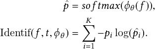 | (7.1) |
where t is the target class, p is the predicted probability, and pi is the target probability. K is the total number of classes and is set to 576.
The verification loss directly takes two descriptor vectors f 1 and f 2 computed from two images as inputs. We compute f s = f 1 �f 2 . After this, we stack several fully-connected layers and add the softmax classifier to project f s to a 2-dim feature vector, representing the predicted probability of whether the two images come from the same vehicle or not. It, therefore, regards the ReID problem as a binary classification problem where the cross-entropy loss function is similar to the classification model. The cross-entropy loss in the verification loss is as follows:
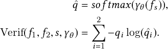 | (7.2) |
where f 1 and f 2 are two tensors of size 1 � 1 � 512. s is the target category indicating the same or different target. �� denotes the whole operation that maps f s to the 2-dim feature vector before the softmax layer.
The verification loss is directly trained on the similarity between two features through an intuitive pairwise comparison method. The disadvantage of the verification loss is that only the verification result is considered in training, while the annotation information is not fully utilized. Also, the association information between the image pairs and other images in the dataset is not utilized.
The classification loss regards the vehicle ReID task as a classification task; each vehicle signature with the same identity is regarded as a category. The classification loss learns directly from the input image and its identity ID. The inputs of the classification model are independent. Still, a potential association relationship is implied because each signature has an implicit relationship with a signature with the same identity and a signature with different identities through category tags. The biggest flaw in the classification model is that the training target is entirely different from the test process. The embedding features are extracted and used to compute the similarity during the test. However, the similarity measurement information between the image pairs is not considered during training.
We have visualized the sum of several activation maps. The classification and verification networks show different activation patterns for vehicles. The ReID network often finds a discriminatory part if only one loss is used. Our proposed model takes advantage of the two networks, and the new activation map is mainly a combination of two separate maps. The proposed model enables more neurons to be activated. In Figure 7.6, we show some examples of the two-dimensional visualization of the embedding.
During training, we resize our input images to 256 � 128, shuffle the dataset, and use a random order of images. Then, we sample another image from the same (or different) classification ID to form a positive (or negative) pair. Initially, the ratio of the negative pair to the positive pair is 1 : 1. We gradually multiply the ratio to reduce the forecast bias until it reaches 1 : 4. This is beneficial because the number of positive pairs is minimal, and the network runs the risk of overfitting. We set the total training epochs to 75 and a batch size of 32. The training begins with an initial learning rate of 0.001 and decays the learning rate to 0.0001 in the last five epochs. Stochastic gradient descent (SGD) is used to update network parameters. The weight of the verification loss is set to 1, and the weight of the two classification losses is set to 0.5. The dropout layers are applied as well.
Given a 256 � 128 image in the testing phase, we feed it to our trained network and obtain the vehicle descriptor f . We obtain another descriptor, f flip, by feeding its horizontal-flipped image. f and f flip are averaged to form the final descriptor. After obtaining the descriptor of the candidate set (gallery set), we save it offline. For the query image, the descriptor is extracted instantly and calculated with the features of the candidate set (query set) to obtain the final matching result.
We propose an effective, fast multi-camera vehicle tracking strategy to speed up the matching process and obtain more stable synchronization results using intersection and other information. The signal data are used before ReID to group local tracklets, e.g., dividing tracks into phases based on green light timestamps.
Based on signature ReID features and temporal cues, we build our track descriptors with a bag of information: signature_match, camera_ID, timestamp, original_track_ID, and class (car, bus, etc.). We first compute the distance matrix using track descriptors as follows:
 | (7.3) |
where ti and tj are track descriptors, and N is the total number of tracks of single-camera tracking from all intersections. We set a very high value for vehicles in the same camera images for the distance matrix because they are not supposed to be merged. We use one predefined threshold for track merging.
Given the distance matrix distanceN, we update the previous multiple object tracking result T following these rules:
where Ti represents a gallery of small tracks with tracking function ID i and qi represents small tracking queries with tracking ID i.
At intersections, vehicles can go in multiple directions. It is more efficient to detect the trajectory direction and then apply ReID and multi-camera tracking. Our dataset has three intersections, A, B, and C, in a corridor. They all have one fisheye camera, and A and B have another pan camera. We filter out tracklets using trajectory direction detection (go-straight, turn-left, or turn-right) and only focus on one direction (e.g., traffic flow go-straight from camera A to camera B then camera C.
Without loss of generalization, for the rest of this chapter, we focus on one-direction tracking for vehicles as they appear at intersection A, then intersection B, and then intersection C. We apply a simple direction detection method based on trajectory information and intersection topology.
We assume that
Since the videos are synchronized, we can compute travel time based on arrival and departure timestamps from final across-camera tracking results:
 | (7.4) |
In the overall pipeline, the single-camera tracking generates tracklet results with information such as camera ID, video_start_time, frame ID, track ID, class, width, height, x, and y. The signal data provide phase information (red or green light), and we use it to group a subsequence of tracklets to one phase. So for signature ReID, the input is a signature representation that includes the image (cropped from detection bounding boxes), track ID, camera ID, frame (departure time), class, and phase ID.
The pairwise matching windows are about 2 phases that usually contain 4-min video data with about 20 to 30 vehicles for one direction per camera. The ReID model outputs the matching results under constraints: (1) the similarity score is higher than the threshold, (2) two signatures are from different camera IDs, and (3) if multiple matching is computed, compute the phase matching matrix (matching phase ID for all signatures in the same phase) and add a penalty for matching results where the matrix distance is larger. We obtain the matching results and use them as registration information for cross-camera tracking for multiple local tracklets. Finally, we have across-camera tracking results with information to compute travel time: start intersection, end intersection, signature ID, departure_time, and arrival_time. We also implemented a visualization part of travel time distribution to aid travel time analysis.
In this section, we first introduce our dataset and experiment settings. Then, we present qualitative and quantitative experimental results.
The experiments were performed on a 256-GB RAM machine with 16 CPUs and 1 NVIDIA graphics card (Titian V). Our signature ReID was implemented on Pytorch. We train a ResNet-50-based signature discriminator on the VeRi dataset as the pretrained model and evaluate our dataset collected from pan and fisheye cameras of corridor intersections in Florida. The VeRi dataset contains over 50,000 images of 575 vehicles captured by 20 cameras. The threshold we set for the signature discriminator is 0.7.
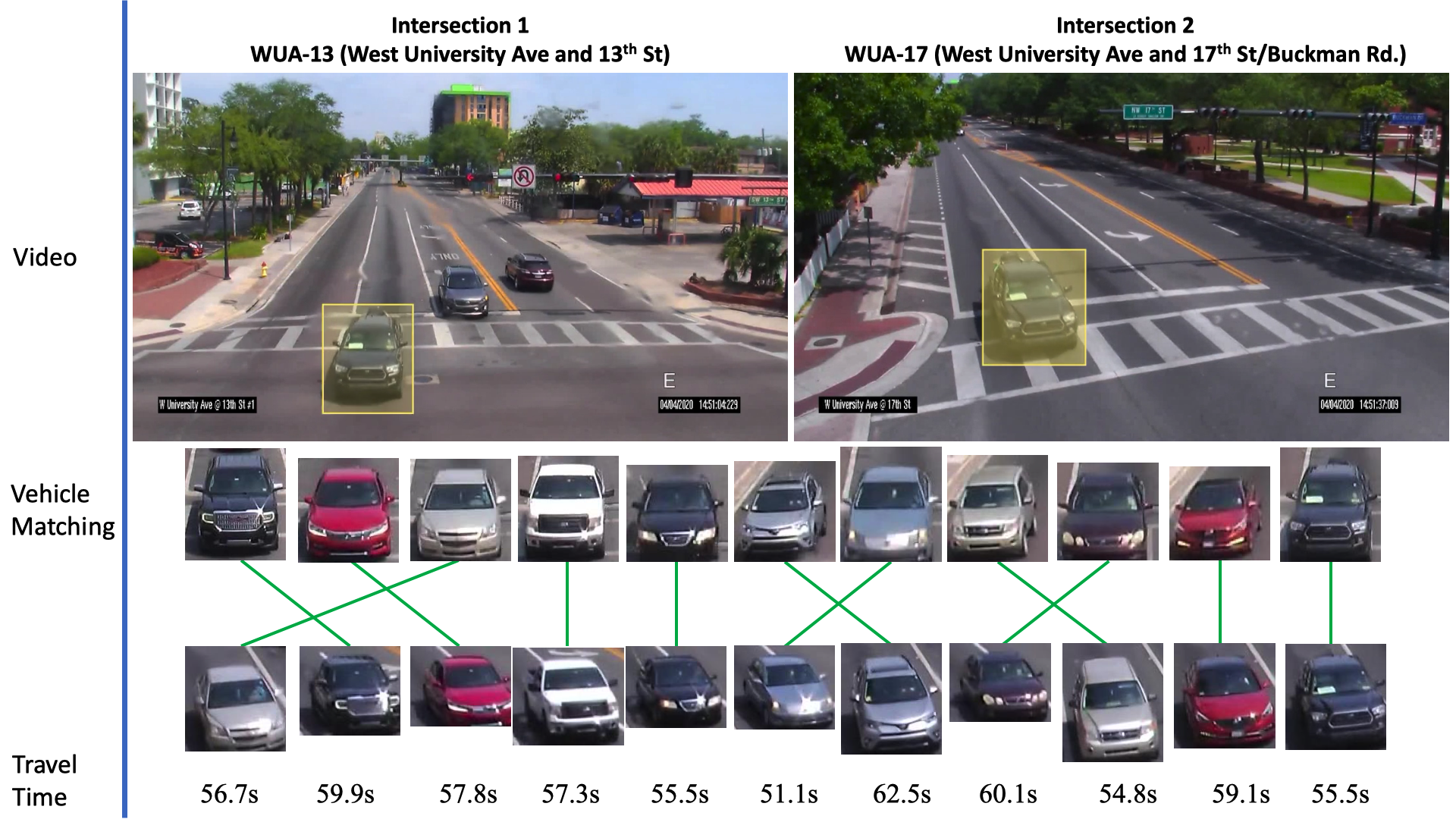
| Figure 7.7.: | Multi-camera tracking and travel time estimation results. Results of one-phase data after first-order matching, sequence order checking, and travel time estimation. Multi-matching did not happen, but sequence order changes. The travel time between these two intersections ranges from 54 to 62 seconds. |
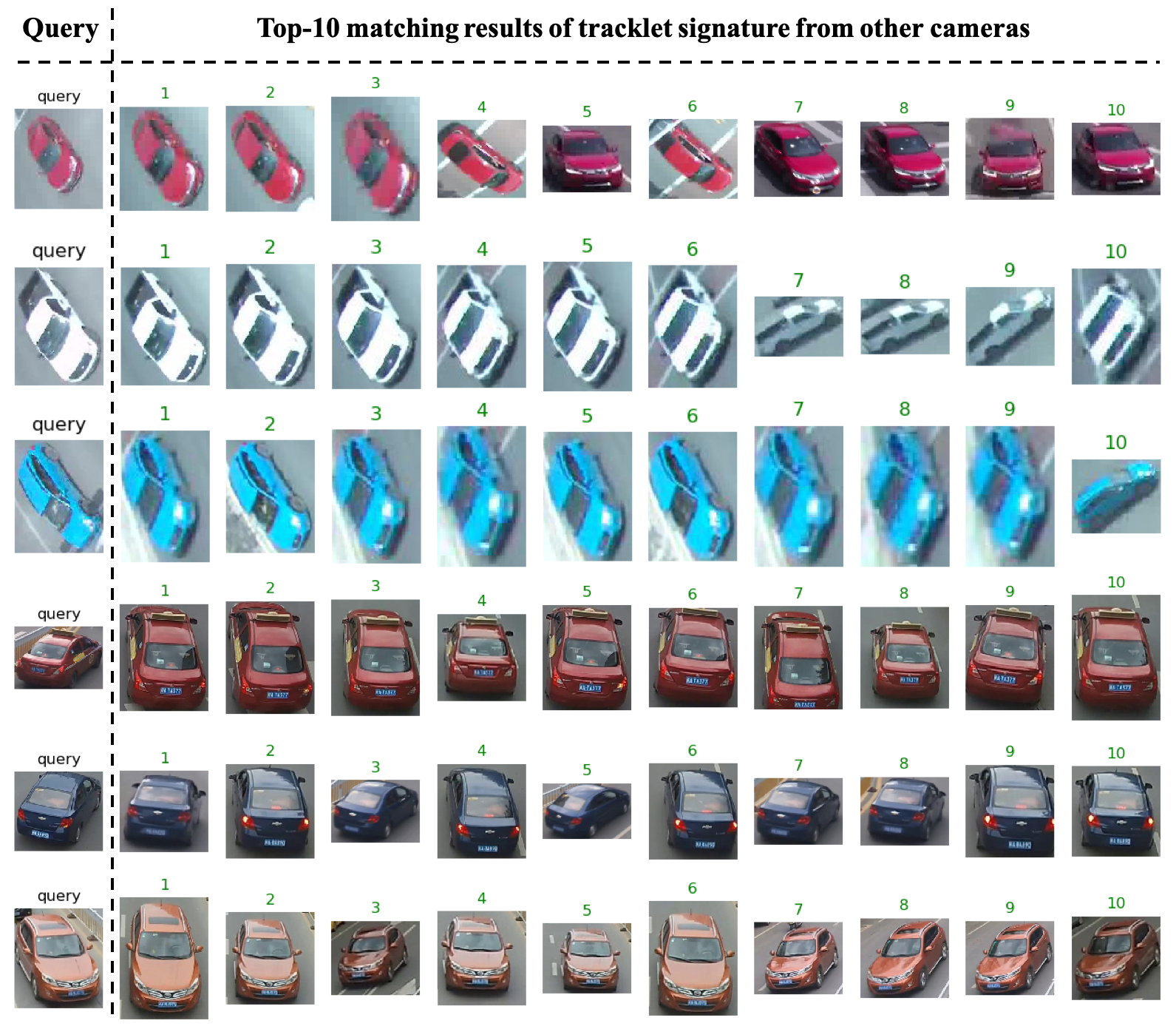
| Figure 7.9.: | Samples of Top 10 matching results of signature ReID on our dataset (top 3 rows: pan+fisheye cameras) and VeRi dataset (bottom three rows). |
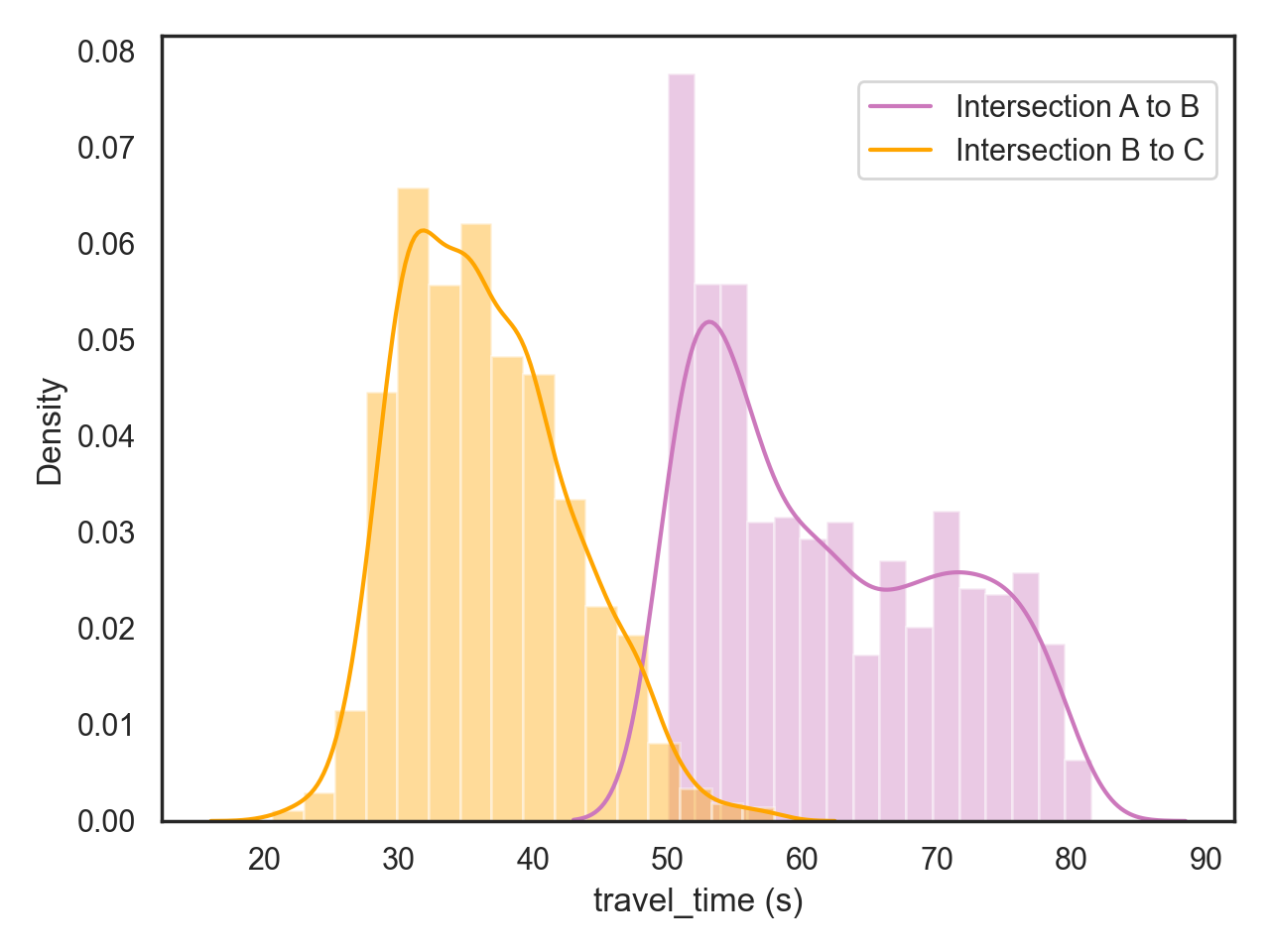
| Figure 7.10.: | Travel time distribution between Intersections A and Intersection B (yellow) and Intersections B and C. (gray) |
The data we used in this method is pure traffic video data collected from three intersections in a corridor in Gainesville, Florida. We refer to the three intersections as A, B, and C. A and B have one fisheye camera and one pan camera, while C only has one fisheye camera. The input of multi-object multi-camera tracking is the M video sequence from M cameras. Since we have two types of cameras, we have two tracking channels: (1) in the fisheye channel, the input is three video sequences from three fisheye cameras, and (2) in the pan channel, the input is two video sequences from two pan cameras.
We evaluate our method using a self-curated video dataset from Intersections A, B, and C. The resolution of pan camera video files is 1280 � 720, and that of the fisheye camera video files is 1280 � 960. The duration of the video files is about 16 to 20 mins, containing approximately 8 or 9 phases. Our test set contains over 200 image sets with over 2,500 vehicle detections. The vehicle types of the test set include cars and buses. Based on single camera tracking results, the signature of each vehicle consists of the detection image (cropped from bounding boxes), camera ID, frame ID, and track ID. Each vehicle has about 11 images (near departure time) per camera, and we can apply a multi-query matching setting by averaging these 11 images for signature ReID.
We present qualitative results of signature matching. We visualize the sum of several activation maps of features from our signature-matching network. As shown in Figure 7.6, the signature ReID network shows different vehicle activation patterns. In Figure 7.7, we present sample results of cross-camera tracking with estimated travel time. In this example, all vehicles that are going straight (left two lanes) in Intersection A (designated as Intersection 1 in the illustration) have correct signature matching at Intersection B (defined as Intersection 2 in the illustration). During this phase, for the group of vehicles (11 vehicles), the average travel time is about 57.3 seconds. We present examples of pairwise signature matching results in Figure 7.8, demonstrating good matching for both fisheye and pan camera data. In Figure 7.9, we show examples of the top 10 matching results for queries from our and the VeRi datasets. Our gallery dataset includes pan and fisheye cameras to compute the top 10 matching results. The experimental results show that our discriminator network has reasonably high accuracy in retrieving correct matching.
To evaluate our signature ReID network, we first evaluate our test dataset with accuracy in terms of Rank-1, Rank-5, Rank-10, and mean average precision (mAP). The definition of mAP is as follows:
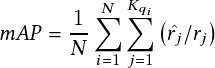 | (7.5) |
where query dataset is denoted as Q =  with N images and gallery dataset is denoted as G =
  with M images. For each query qi, we sort the gallery data in ascending order of ReID distance and denote the sorted gallery as Gqi and the matching subset in Gqi as Ĝqi =
  . Assume gj in Gqi has index rj, in Ĝqi has index rj, we repeat this query processing for all query data. Rank-1 is defined as rank1 = N�N where qi meets Rank-1
if the first match is correct in Gs of qi. The number of queries that meet Rank-1 is Q is N.
. Assume gj in Gqi has index rj, in Ĝqi has index rj, we repeat this query processing for all query data. Rank-1 is defined as rank1 = N�N where qi meets Rank-1
if the first match is correct in Gs of qi. The number of queries that meet Rank-1 is Q is N.
We train our signature ReID model on 576 training sets from the VeRi dataset and test it on our dataset with 200 testing sets (including both pan and fisheye data). The test and training datasets were disjoint. Table 7.1 shows that we have outstanding accuracy in both single-query and multi-query settings in terms of Rank-1, Rank-5, and Rank-10. The mAP of 0.853039 for a single query is also good. A quantitative prediction of single camera tracking, pairwise signature ReID, and phase-based signature ReID is achieved by comparing predicted results with the ground truth at the frame or object levels. We apply a predefined threshold (e.g., 0.7) to compute matching candidates and pick the highest score for the final results. A true positive is a match where the object signature IDs are the same, but the camera IDs are not the same. A false positive occurs when the object signature IDs are not the same. A false negative occurs if there is no match with ground truth and matching results. The precision, recall, and F1 score are defined as
 | (7.6) |
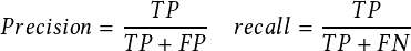 | (7.7) |
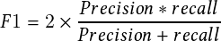 | (7.8) |
The evaluation metrics we used for quantitative evaluation include precision, recall, F1 score, and speed for the four major modules of the proposed method. Table 7.3 shows that our pipeline has achieved promising performance on three modules: single camera tracking, pairwise signature ReID, and phase-based signature ReID. Figure 7.10 and Table 7.2 shows the test set’s travel time distribution and statistics information. The distribution of travel times between Intersections A and B shows two spikes for this road segment. It aligns with our investigation: the first vehicle queued in the lane influences the actual travel time of that group of vehicles.
The signature ReID performance in both single-query and multi-query settings is shown in Table 7.1. The ReID model training takes about two hours on our device: one NVIDIA Titan V. In Table 7.4, we present the processing time of each component for a 5-minute video clip (1280 � 960, 10 fps). The overall pipeline costs 221 to 237 seconds and achieves real-time performance.
| Table 7.1.: | Quantitative evaluation of our discriminator for signature ReID matching |
| Component | Single Query (re-ranking) | Multi-Query
| ||||||||
| Task | Dataset | Loss | mAP | Rank-1 | Rank-5 | Rank-10 | Rank-5 | Rank-10 | ||
| ReID | VeRi | Classification | 0.67 | 0.91 | 0.93 | 0.96 | 0.88 | 0.95 | ||
| ReID | VeRi |
| 0.72 | 0.94 | 0.96 | 0.98 | 0.94 | 0.97 | ||
| ReID | Ours | Classification | 0.79 | 0.89 | 0.89 | 0.92 | 0.85 | 0.85 | ||
| ReID | Ours |
| 0.85 | 1.00 | 1.00 | 1.00 | 0.96 | 1.00 | ||
| Table 7.2.: | Travel time computation results |
| Intersections | Mean of Travel Times | Standard Deviation |
| A to B | 61.80 s | 9.03 s |
| B to C | 36.55 s | 6.18 s |
This chapter introduces a novel method and a real-time system to estimate vehicle travel time by leveraging video processing on multiple intersections.
Our key contributions can be summarized as follows: (1) we propose a novel video-based signature ReID method with high precision that plays a crucial role in multi-camera vehicle tracking; (2) we introduce a novel way to extend pairwise signature matching to phase-based signature matching to tackle the sequential group signature ReID problem on traffic video datasets; and (3) we propose a real-time video processing system for multi-camera vehicle tracking and travel time estimation; We evaluated the proposed framework on a real-world dataset from intersections in Florida with pan and fisheye cameras. Although our results were presented for three intersections, the pairwise intersection nature of our approach allows for scaling this approach to a larger number of intersections. Overall, our experiments demonstrated the proposed approach’s viability, effectiveness, and scalability. Our future work will extend this to computing origin-destination travel times to all pairs of inputs and outputs across all intersections in a corridor or a traffic network.
Most traffic intersections today have different sensors, such as video cameras, lidar units, and traditional induction loop detectors. Technological advances enable us to monitor these intersections remotely in real time and identify potential inefficiencies. However, the high volume of data being collected by the sensors at each intersection and the number of such intersections in a city makes it imperative to automate the process of monitoring and analyzing problem areas. Using state-of-the-art machine learning algorithms and data communication mechanisms at the back end, we have developed a visual analytics system to study the videos generated at an intersection.
The system can detect movement conflicts or near-misses in streaming mode within a small latency. The system also can perform historical analysis where the user specifies a time window of interest. The tool may filter and analyze the trajectories of vehicles and pedestrians passing through a traffic intersection during that time. The system is based on intersection videos obtained using fisheye cameras because fisheye cameras can capture a complete view of the intersection, unlike regular cameras that can record approaches from only one direction.
The main contributions of our work presented in this paper are summarized below.
A user interface (UI) was developed in [70]. Apart from the fact that the infrastructure is completely different for the two systems (the new system is Web-based, while the system in [70] is based on Qt), we have incorporated many new features in the new system. Some of these features are summarized here:
The rest of the chapter is organized as follows. Section 8.2 presents the related work in trajectory analysis. Section 8.3 gives preliminary background on video processing. Section 8.4 shows the core of our visualization software. Section 8.4.2 is devoted to the historical analysis mode of our visualization software, and Section 8.5 presents a trend analysis case study. We finally conclude in Section 8.6.
The field of trajectory analysis for pedestrians and vehicles has become a hot area of research after the advent of intersection cameras. However, only some existing works have developed a complete analysis framework and a user interface for analyzing the videos. In this section, we mention some work that closely resembles our work in this book regarding the components that build the analysis system. Sha et al. [168] performed trajectory analysis using laser data obtained from objects using an intersection. Xu et al. [169] present an algorithm for clustering the trajectories at an intersection. In our work, we have developed visual analytics software on top of the analysis algorithms.
TrajAnalytics [170] is an open-source visual analytics software developed by Dohuki et al. TrajAnalytics is used for exploring urban trajectories and has built-in algorithms to perform modeling, transformation, and visualization of urban trajectory data. A fundamental difference between TrajAnalytics and our visual analytics system is that the software analyzes the whole trajectory of vehicles and pedestrians in the former. In contrast, we analyze only trajectory segments that appear at traffic intersections.
Another existing tool developed by Kim et al. [171] performs analysis at different stages, such as map view, trajectory view, analysis view, and timeline view. The tool provides the user options to filter areas of interest in the map view, generate the trajectories of interest, and study the timeline of these trajectories. This work also analyzes entire trajectories from start to end, and hence, their data collection mechanism and software content and features are very different from our software.
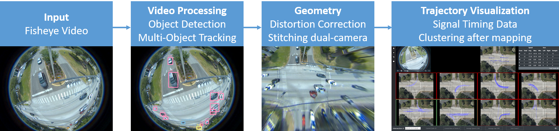
| Figure 8.1.: | An overview of the pipeline consisting of video processing and multi-object tracking for trajectory generation, followed by post-processing and fusion with signal data, and finally, visualization. |
In this section, we describe some preliminary concepts fundamental for trajectory generation from raw videos. Figure 8.1 demonstrates the video processing pipeline. Using computer vision techniques, we process the raw fisheye videos and detect and track objects at an intersection, such as cars and pedestrians. We cluster the generated trajectories as a post-processing step before visualization.
Video analysis deals with the algorithms needed to process the raw videos to generate trajectories. Our software has been developed to process videos from fisheye cameras, but it can easily be extended to process videos from ordinary cameras. The benefit of using a fisheye camera is that it can capture the whole intersection in a wide panoramic and nonrectilinear image using its wide-angled fisheye lens. This allows a fisheye camera to capture the entire intersection in a single view. In some cases, where the intersection is large, two or more fisheye cameras are often used to get a complete picture.
Detecting and tracking objects using timestamped coordinates leads to the generation of object trajectories. For a typical intersection that is moderately busy, there are over 10,000 trajectories happening on a weekday. Thus, a visualization system helps monitor traffic behavior automatically without watching traffic videos. In our software, we automatically anonymize the information about the moving object by saving to our database only the location coordinates of objects and, in the cases of vehicles, their size and color.
As a result of video processing, a video is converted to a series of frames. The objects are detected and tracked across the frames in all of these frames. Video processing uses a temporal superpixel (supervoxel) method [61] to extract an accurate mask for object representation. These can be converted into trajectories representing traffic’s spatial and temporal movement. A trajectory is a path traversed by a moving object represented as successive spatial coordinates and corresponding timestamps. The details of our video processing and analysis system are presented in detail in [73].
We use a relational database in the cloud to store the trajectories generated by our software and the signal phase and timing information obtained from high-resolution controller logs. Figure 8.2 presents the key attributes found in the database. The attributes of TrackInfo represent the properties of the trajectories we consider for analysis. These are (1) frame_id, which identifies the current video frame, (2) track_id, which determines a trajectory, (3) x and y, the coordinates of the object location, (4) w and h, the width and height of the bounding box enclosing the object, (5) intersection_id, which identifies the intersection, and (6) date and time, which represent the timestamp. Correspondingly, the attributes for signal data include (1) intersection_id, (2) timestamp, (3) the current state of the signals encoded in a hexadecimal format, (4) the cycle number (relative to the cycle number of the first observation), and (5) camera_id, which is an additional attribute that depends on the intersection.
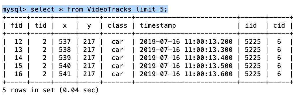
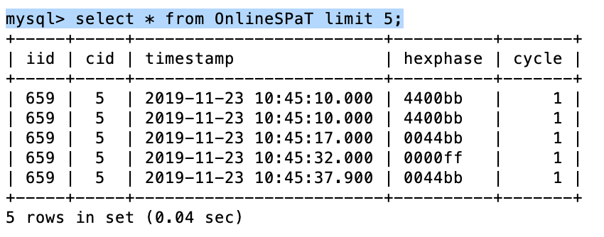
| Figure 8.2.: | MySQL databases of trajectories generated by video processing (left) and the signal information (right) generated from ATSPM. |
Given a video feed, one of the first tasks is to generate the trajectories. We summarize the steps involved in generating the trajectories here. Each trajectory is preprocessed to eliminate coordinates that appear outside the intersection scope. This step is helpful because trajectories farther away from the fisheye cameras tend to be noisy. After the preprocessing, we fuse the signal timing data with the tracks. An unsupervised clustering approach is used to cluster the trajectories as a final step.
Because we focus on capturing trajectories through an intersection, we observe a definite pattern of movement brought about by the presence of through and turn lanes and the signaling system at an intersection. The advanced transportation controllers (ATCs) allow us to record the exact time for signal changes and detector on/off events 10 times a second. We download the recorded data for the intersection for a given period.
The signal controller records the signal changes to an intersection’s red, yellow, or green light. We store the current intersection state in which signals are red/yellow/green using a 24-bit binary number and its hexadecimal equivalent. This encoding works out as follows: we divide the 24 bits into three sets of 8 each. The first set of eight bits is reserved for recording the green status on each phase. The green status may be ON(1) or OFF(0) for each phase 1 through 8. Similarly, the second and third sets of eight bits are reserved for recording yellow and red status, respectively. This encoding is explained in the following example. Suppose phases 4 and 8 are green, and every other signal is red. Then the 24-bit signal state is 0001 0001 0000 0000 1110 1110. The equivalent hexadecimal representation is 1100ee.
So, now we have two sets of data: video and signal phasing data. Our next step is to fuse the data and annotate each trajectory coordinate with the signal state when it happens. This is possible because the video processor annotates each trajectory coordinate with the timestamp when that coordinate is traversed. Thus, upon starting to process a new video, the first thing is synchronizing the video timestamps with the controller timestamps. The video processor’s timestamps are usually a few seconds later than those on the controller logs. The offset results are due to the time difference between starting the command and receiving the video stream.
For clustering the trajectories, we need a distance measure that is appropriate for the trajectories. We developed a distance measure based on FastDTW [172] to compute a list of coordinate pairs from the two trajectories that align with each other while considering the different trajectory speeds. FastDTW approximates the dynamic time warping algorithm to find the optimal alignment between two-time series with near-linear time and space complexity. To compute the distance between the trajectories, we use the coordinate alignment pairs from DTW to divide the space between the trajectories. Then, we calculate the sum of the area of the triangles and divide it by the average length of the two trajectories to determine the average distance between the trajectories.
Following the computation of the distance between every pair of trajectories, we apply spectral clustering to obtain the trajectory clusters.
Our visualization software is divided into two parts: the frontend and the backend. The frontend is written in Vue.js, one of the most popular progressive frameworks for building user interfaces. The frontend has two modes: the streaming mode and the historical mode. The streaming mode loads the video and corresponding starting timestamp from the backend, then uses a cache to query the database every 5 seconds for three operations: track animation, the statistics related to the tracks, and the display of tracks by phases. In the historical mode, on the other hand, the software reads the database based on filters that the user can select. The backend is written in NodeJS, whose primary purpose is to query the database. The backend loads the Ajax post from the frontend, then queries the database using the received data. The backend also prepares the video file or stream to be displayed in the frontend. We now describe the capabilities of our software in more detail, first for the streaming mode visualization in Section 8.4.1 and then for historical analysis in Section 8.4.2.
A data flow diagram (DFD) describes the software’s overall structure. The diagram Figure 8.3 shows how the data goes through the pipeline and finally appears in the interface.
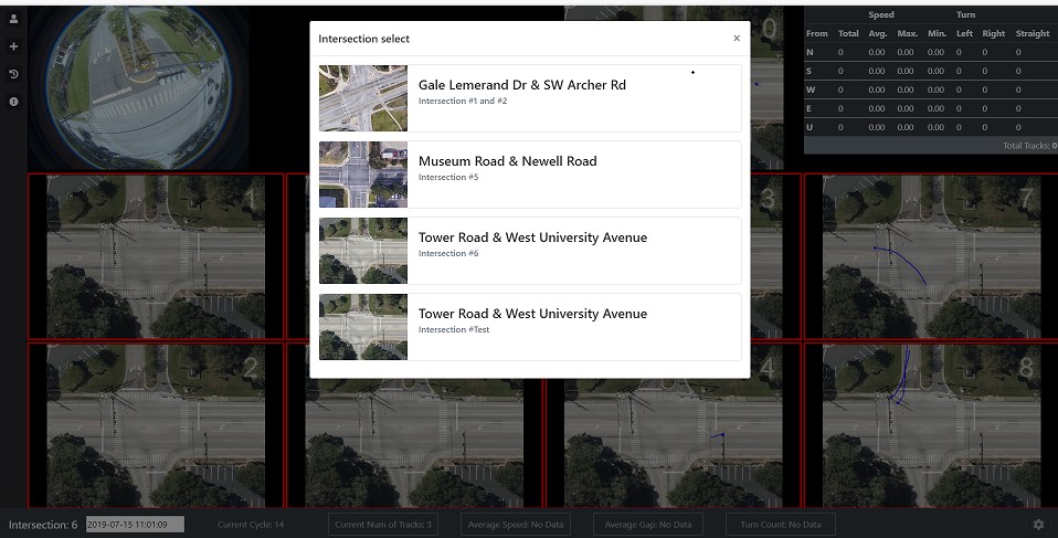
| Figure 8.4.: | The selection of the current intersection can be opened by clicking on the button on the sidebar. |
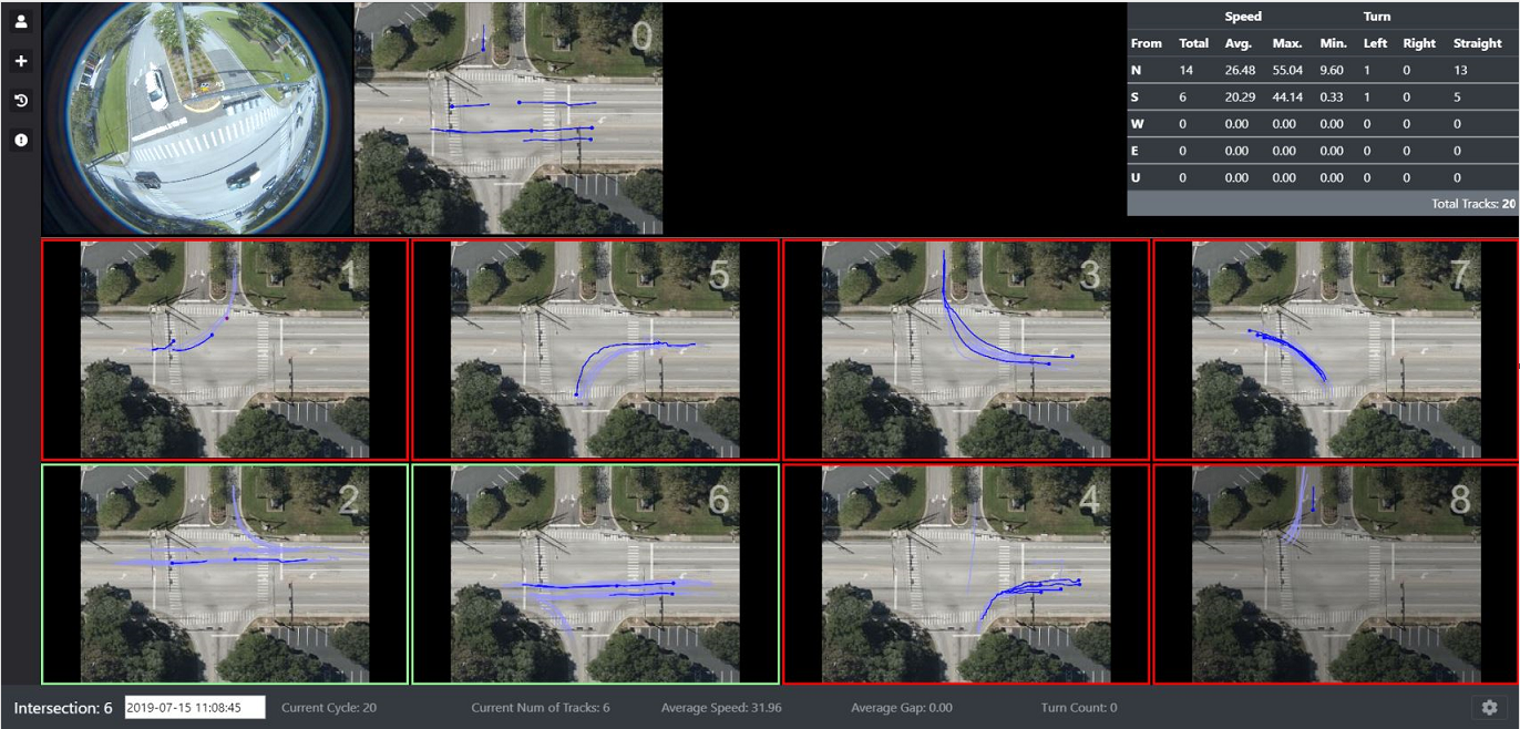
| Figure 8.5.: | Interface for processing streamed tracks. The video from the fisheye camera is at the top left corner. This is followed by an unwarped image of the intersection and the trajectories represented by a moving dot. The statistics of the trajectories on the intersection are captured in the table on the top right side. The trajectories are partitioned into phases and displayed in the eight windows. The setting options and average statistics about the trajectories are presented at the bottom. |
After connecting to the tool, the user logs in and chooses the intersection of interest. The intersection selection step is shown in Figure 8.4. The tool supports the analysis of multiple intersections simultaneously. The streaming mode page, as shown in Figure 8.5, is the first page the user sees after logging into the system and choosing the intersection of interest. The various components of this page are described below.
The fisheye video of the intersection, as captured by a fisheye camera, is streamed or played on the top left corner of the Web page. An animation of the object trajectories is created by representing the objects as moving dots at the intersection. This animation is displayed beside the video in an unwarped space and in a time-synchronized manner for the actual video.
For streaming mode accessibility of the data, we use database caches or put the data in memory where appropriate. In other words, we use a buffer to store all the data we get from the database. We set a timer to read the max timestamp stored in the buffer while comparing it with the current timestamp obtained from video play. Once the max timestamp of the buffer is less than 5 sec later than the current one, the program queries the database and reads 5 sec of data after the max timestamp. Thus, 5–10 sec of future data is stored in the buffer every time. As the buffer size increases, the timer evicts the last hour of data when the total data reaches three hours. A pointer for the start point of the tracks updates every animation frame for a faster query of animated tracks.
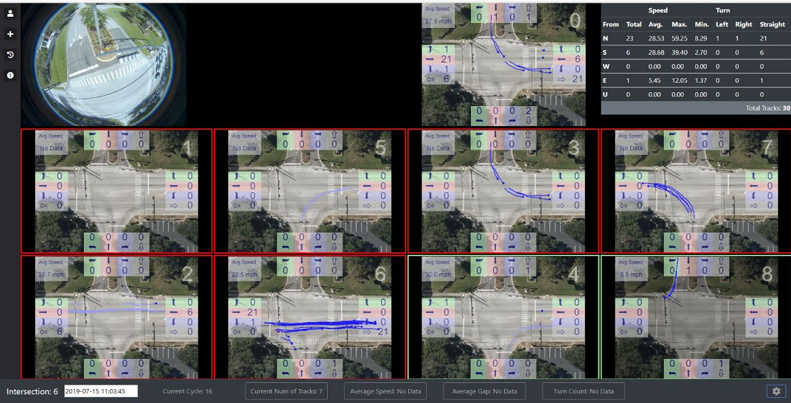
| Figure 8.6.: | The overlay feature of the tool may be used to display the vehicle egress and ingress counts for the different phases of movement. |
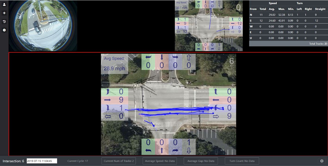
| Figure 8.7.: | A particular phase was zoomed in by clicking on that phase from the main page. The user can toggle to the main page by clicking the zoomed-in phase. |
There is a window for each of the eight phases of traffic movement, as shown in Figure 8.5. The eight windows are tiled and numbered according to the phase they represent. An ongoing trajectory is assigned a phase by first performing matches with the existing centroids or cluster centers. The trajectory phase is set to the phase of the matching centroid.
After the phase is assigned, the trajectory is displayed in the respective phase window. Separating the trajectories by phases makes them easy to track and helps us count the number of vehicles and their classes for each movement. The software supports an overlay on the phase windows that displays the number of vehicles in the through and turn lanes for that movement for a given time window, shown in Figure 8.6. The user may enable the overlay by clicking on the settings and then toggling the “Enable Overlay” switch.
It is possible to zoom in on only one phase by clicking on that phase. The result is shown in Figure 8.7, where phase 6 was selected by the user,
Our software integrates the trajectories with signal data to place the trajectories in the context of the current signaling state of the intersection. This signal data integration enables us to detect anomalous traffic behavior at the intersection, such as vehicles moving in the yellow signals or those jumping the red. The signal data information in the GUI is displayed by framing each window with a box of the same color as that of the signal for that phase. Phases 2 and 6 are being served in Figure 8.5; hence, these phase windows are framed by green boxes in the figure.
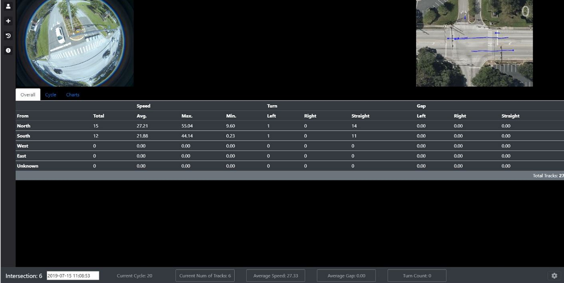
| Figure 8.8.: | Clicking on the statistics table on the main page toggles the display to more statistical details. These are organized into three tabs: Overall, Cycle, and Charts. The overall statistics for speed, gap, and turn movement count are here. |
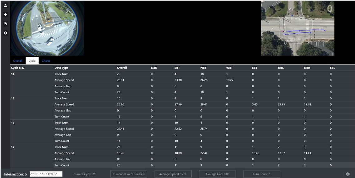
| Figure 8.9.: | The detailed statistical data cycle tab shows the statistics data aggregated by signal cycles and displayed by cycle counts. |
The statistics for the various trajectories are available in the form of charts and tables. The table appears on the top right corner of the streaming page of Figure 8.5. The table shows the most common statistics, such as the number of vehicles or pedestrians for each movement and the average, minimum, and maximum speeds in mph for those movements. If the user is interested in more details, such as the average gap or the response time, the table may be clicked to bring up the details. The further details are organized into three tabs: Overall, Cycle, and Charts, as shown in the Figures 8.8, 8.9, and 8.10, respectively. The Overall tab gives the overall observations, as the name suggests. The Cycle tab aggregates the data on a cycle-by-cycle basis. The Chart tab, on the other hand, shows the overall trend of the characteristics over time.
Our visualization tool displays a merged image from two or more cameras typically installed in a large intersection. Figure 8.11 shows one such intersection, where two cameras are installed in the opposite corners of a large intersection. The animation merges the views from the two cameras and creates a single image.
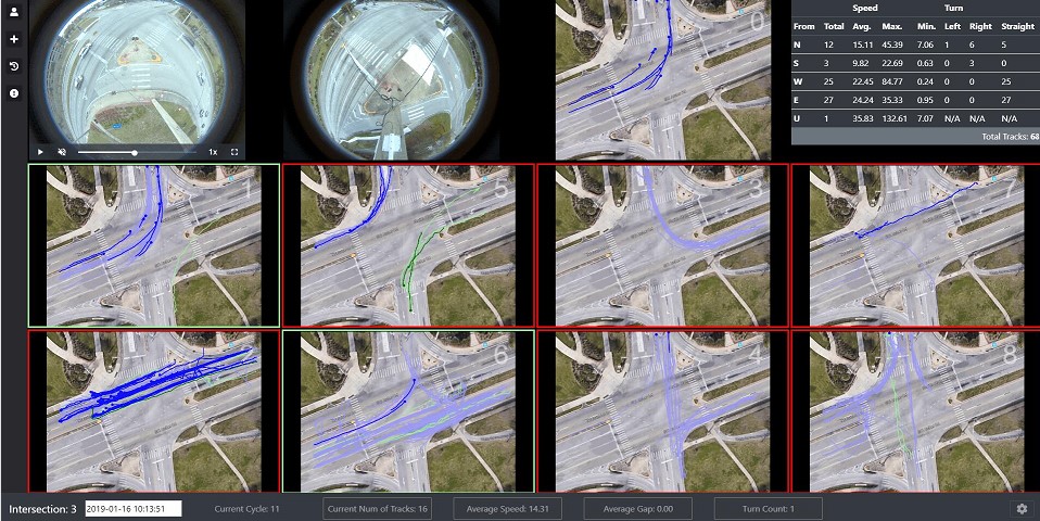
| Figure 8.11.: | The images from an intersection with two cameras. The cameras are installed in opposite corners of the intersection, and the raw video from each camera appears in the top left corner. |
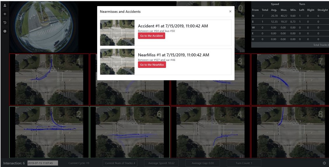
| Figure 8.12.: | The interface for displaying near-miss and crash events in streaming mode. The two events described here are hypothetical and are used to test the interface. |
Our tool automatically picks up the near-miss and crash events and reports separately. Such incidents are usually rare, but Figure 8.12 represents a hypothetical situation to demonstrate the feature.
It is possible to get the track ids of the tracks currently being displayed by clicking on the “Current Num Of Tracks,” which is shown in Figure 8.13. The user can view the detailed information on that path by choosing a track. These include the speed, cluster, and phase of the path.
In addition to the settings of the features described above, there are other valuable features, such as coloring trajectories by object classes or selecting the time frame for displaying tracks, such as those that happened in the last x seconds. Figure 8.14 shows the entire selection collection available to the user upon clicking the settings.
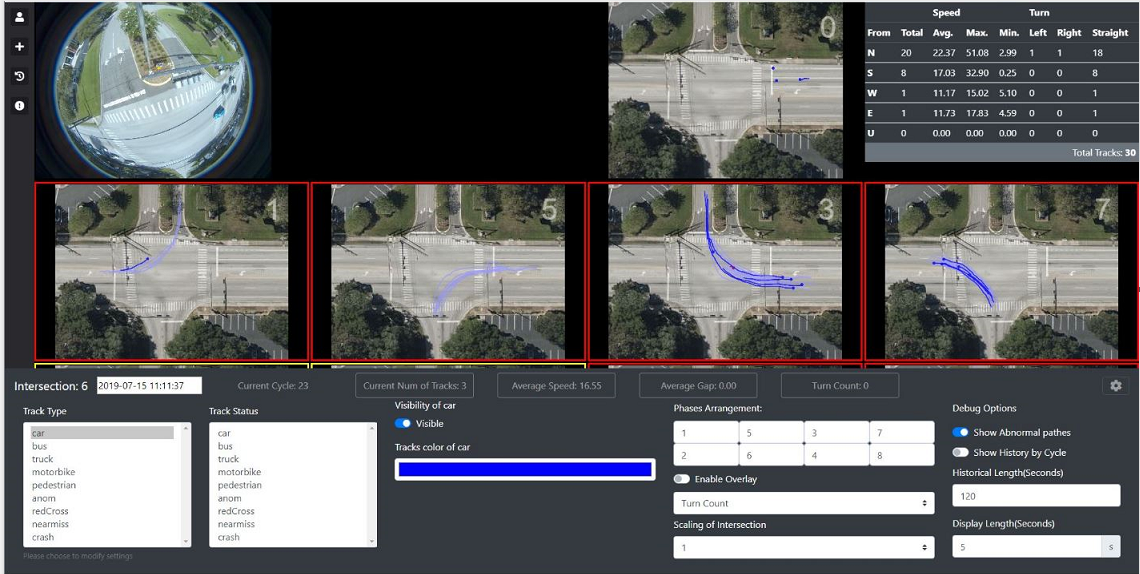
| Figure 8.14.: | The settings menu. It offers several options to the user for enhanced display. It contains the option to enable overlay, set the color for trajectories based on class type, and set the window to display historical data within the streaming mode. The latter is usually set to about 2 minutes to capture all trajectories in an ongoing cycle. |
Our visualization software may be used for mining the trajectories created in the past from traffic videos. In this section, we describe the features supported for historical analysis. Figure 8.15 shows the landing page for historical analysis. It allows the users to filter the trajectories based on time of occurrence, phase, and cluster.
Further, the user may view the cluster centroids of the dominating clusters, the anomalous trajectories, or even filter out the trajectories impacted by noises. It also supports the side-by-side display of trajectories for different combinations of time of the day, the day of the week, or classes of objects. We present some of the possibilities in this section.
The time slider, used for selecting a time window, is the primary filter. It is a range slider with a flexible start and end. Once a time window is chosen, all the trajectories occurring in that time window on the selected intersection are obtained using a database query and displayed on the screen. The trajectories in Figure 8.15 show such an example, where the time window length is 10 minutes starting Monday, 15 Jul 2019, 15:00:12 GMT.
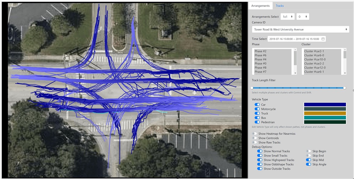
| Figure 8.15.: | The display for historical analysis. It provides several options for filtering a large collection of trajectories. The primary filter is based on the time range. All tracks that happened for 10 minutes starting on Monday, 15 Jul 2019, 15:00:12 GMT, are displayed here. |
All trajectories in a given time window may be further partitioned based on their movement and cluster. Figure 8.16 shows all the eight phases the trajectories are partitioned into for the trajectories belonging to the time window chosen in Figure 8.15. The top left window shows all the trajectories, whereas the other windows show the trajectories corresponding to the eight vehicle phases described in [69].
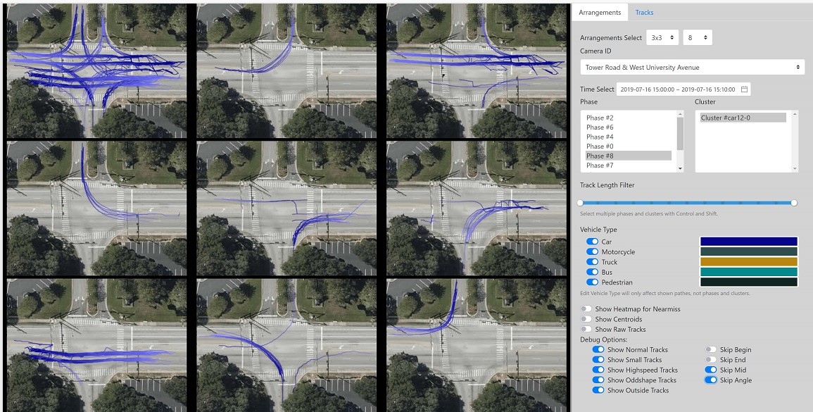
| Figure 8.16.: | The tracks in the top left corner are partitioned into different phases. Going row-wise from top to bottom and from left to right of each row, the first window on the top left corner shows all the tracks in the previously chosen time range. Then the tracks for phases 1, 2, 3, 4, 5, 6, 7, and 8 are displayed on the respective windows. |
Figure 8.17 showcases a selection combination for phases and clusters. The trajectories in phase 6 here are partitioned into three clusters. Two of these, namely, ’car6-0’ and ’car6-1’, correspond to the trajectories on the two lanes, respectively, while ’car11-0’ corresponds to the right-turn trajectories. These three clusters are shown in the three remaining windows. The remaining cluster, ’small,’ corresponds to the tiny tracks created due to processing errors and are not shown in this figure. Figures 8.16 and 8.17 demonstrate our software’s powerful feature, enabling side-by-side comparison of sets of trajectories, where each set may be chosen independently using any criteria.
The “Phase” window often has a phase 0, simply a phase to which the trajectories are assigned when the software cannot determine their movement direction. This happens for anomalous trajectories and trajectories resulting from a processing error.
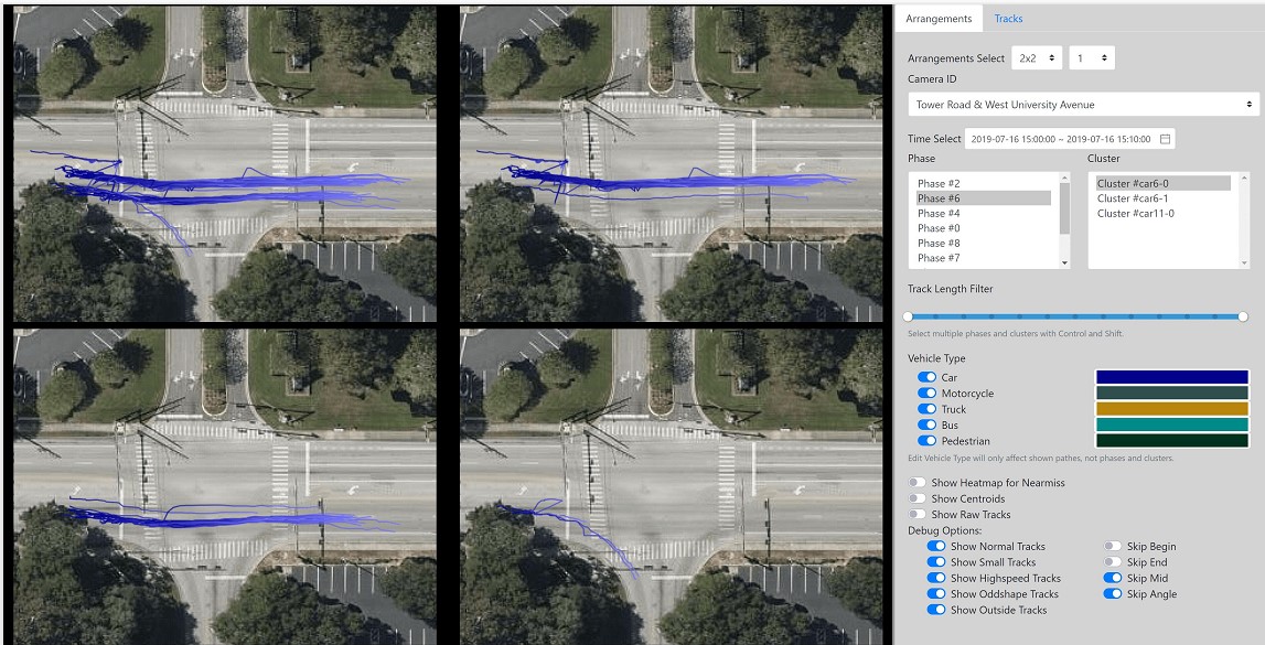
| Figure 8.17.: | A combination of phases and clusters was used to display all trajectories in phase 6 and their respective clusters. These clusters automatically partition the trajectories based on their lane of occurrence and between the through and right-turn trajectories, |
The visualization tool may display the cluster centers used for the online cluster assignment. This is useful in sampling the major movements at an intersection. It also comes in handy in debugging mismatched alignment and stitching small tracks. Figure 8.18 shows the cluster centers corresponding to the trajectories of the 10 minutes duration chosen earlier.
It is possible to filter the trajectories by the object classes, such as cars, buses, trucks, and pedestrians, which makes it easier to generate a count of each type of object for a given time window. Figure 8.19 shows an example of this.
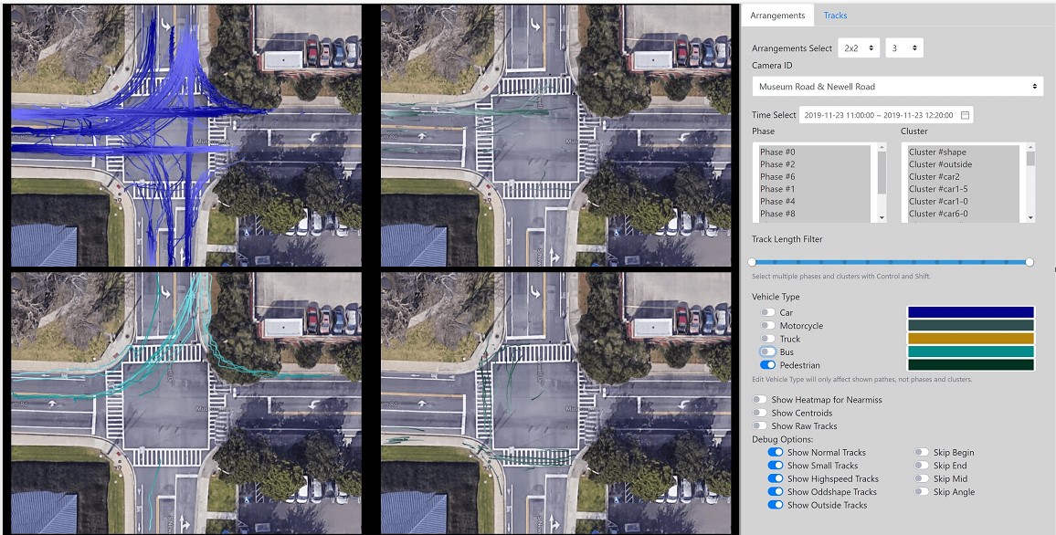
| Figure 8.19.: | The trajectories are partitioned by the object classes. The top left window shows all the trajectories made by cars, the top right window shows the trajectories made by motorcycles, the bottom left window shows trajectories generated by buses, and finally, the bottom right window shows trajectories generated by pedestrians. |
Figure 8.20 shows how heat maps would appear to highlight unsafe areas of the intersection that have had more near-misses. The heatmap in this figure is based on a hypothetical dataset.
So far, we have focused on the display of sets of trajectories. Viewing the individual tracks by choosing a track from the Tracks tab is also possible. Figure 8.21 shows an individual highlighted trajectory. The highlighted trajectory’s details, such as start time, end time, track ID, phase, and object class, are shown at the bottom right corner.

| Figure 8.21.: | An individual trajectory selected by clicking on a track number from the Tracks drop-down. |
A track may be anomalous for several reasons, such as when its shape does not conform to any cluster centroids or occurs while the ongoing signal is red. Figure 8.22 shows the set of anomalous trajectories with a trajectory we have highlighted that turns left from a through lane, even though there is a left-turn lane at this intersection.
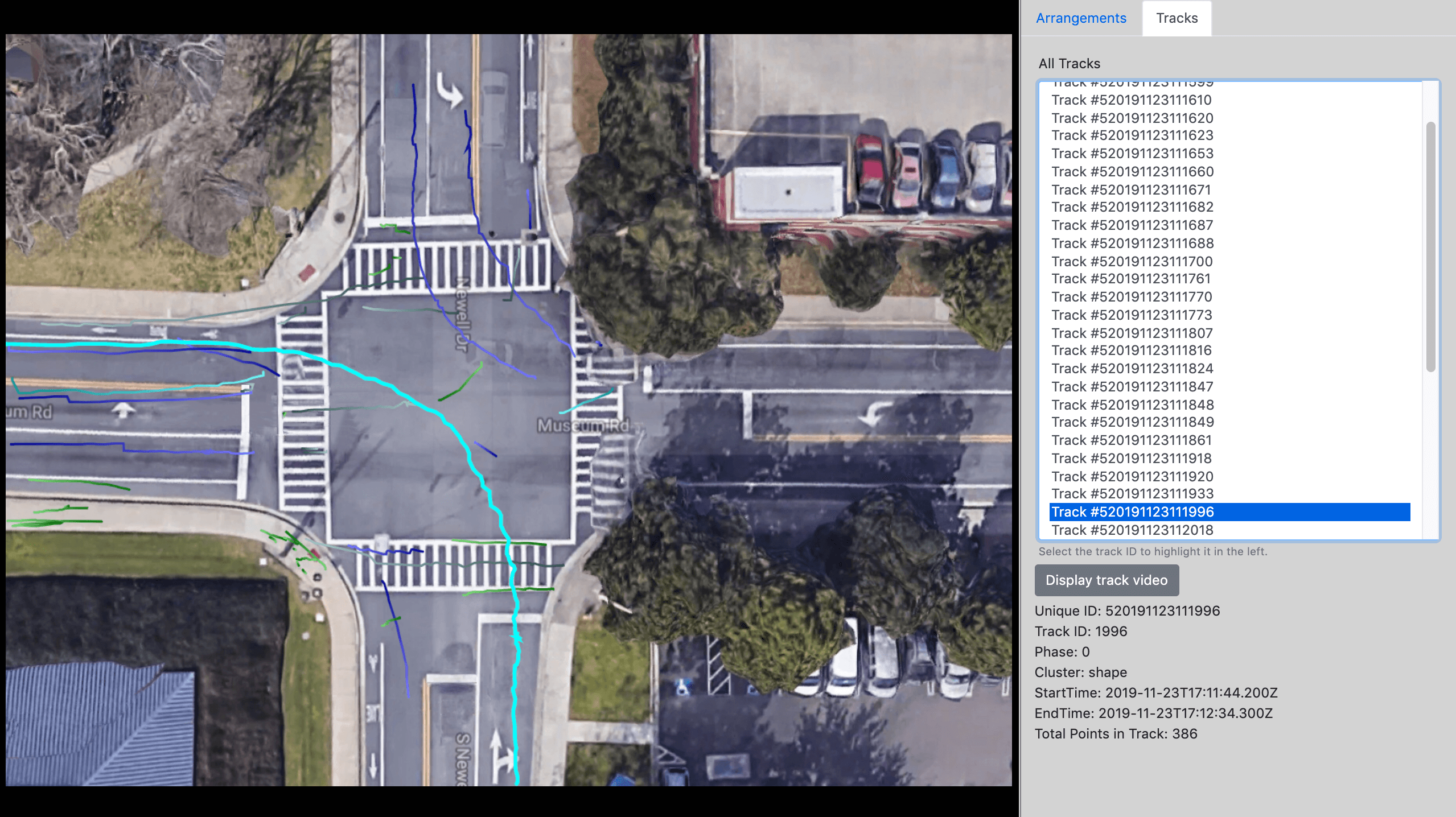
| Figure 8.22.: | All trajectories that are identified as anomalous. The one highlighted takes a left turn from a through lane. |
The software lets the user verify any trajectory in the historical domain by playing its video clip if the corresponding video is available. This feature makes our software an excellent debugging tool for developers because it closes the gap between a trajectory stored as a set of coordinates and the same trajectory as it traversed in a real-life scenario. Figure 8.23 shows a snapshot of the video being played that corresponds to the trajectory chosen in Figure 8.21.
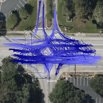
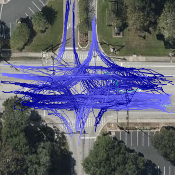
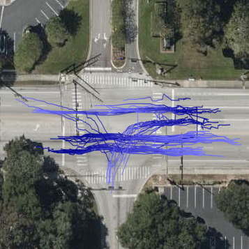
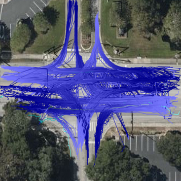
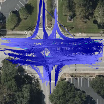
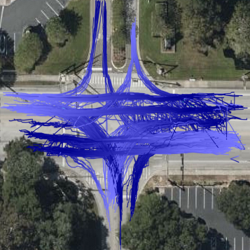
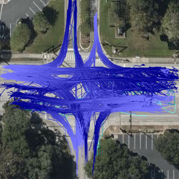
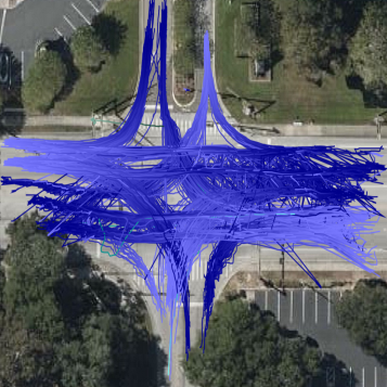
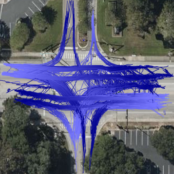
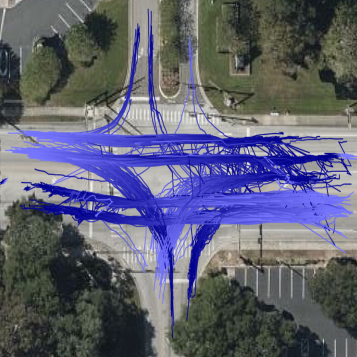
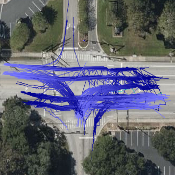
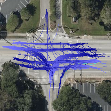
| Figure 8.24.: | A case study for trend analysis. Each of the 12 tiles represents the trajectories over 2-hour intervals over a day for multiple days a week. In particular, the left column of tiles represents a Monday, the middle column represents a Wednesday, and the right column represents a Sunday. Each row of tiles is for a different time of day. The top row is from early morning (7 AM–9 AM), the second row is from late morning (11 AM–1 PM), the third row is from the afternoon (3 PM–5 PM), and the last row is late evening (7 PM–9 PM). |
This section aims to demonstrate how our software can effectively study traffic trends without observing hours of videos. Using the historical analysis interface, we can analyze trajectories from the same time interval over multiple days and discover trends. Trajectories from multiple days may be loaded using the tiling feature described earlier. Figure 8.24 demonstrates the time of day and day of the week trends for the main clusters of car trajectories. The tiles’ left, middle, and right columns are from Monday, Wednesday, and Sunday of a given week. On the other hand, the tiles on each row are from different intervals. The first row from the top shows data for early morning (7 AM–9 AM), the second row of tiles shows data for mid-morning (11 AM–1 PM), the third row for the afternoon (3 PM–5 PM), and the last row shows data from the evening (7 PM–9 PM). Figure 8.25 gives the exact count of vehicles per direction (east, west, north, south) and movement (through, right, left).
We present some observations below based on these comparative vehicle counts by the time of day and week.
In this chapter, we presented a novel software we developed for performing visual analytics. The software is designed to serve the broader user community of traffic practitioners in analyzing the efficiency and safety of an intersection. The software runs video analysis and generates the spatial locations and timestamps of all the objects passing through an intersection along with their object type.
As described in the chapter, our software has two modes: a streaming and a historical mode. These have their own merits and are helpful to a traffic engineer who can quickly analyze the trajectories to better understand traffic behavior at an intersection instead of watching long video sequences. For example, our software can diagnose red-light violations or high traffic in a turning bay. The traffic engineers can test appropriate remedies by performing before-and-after studies, and the problems may be reduced or eliminated.
The software is intuitive and straightforward to use, and it could help study trends in traffic patterns for different times of the day and the days of the week.
The implementation of computer vision and machine learning in Intelligent Transportation Systems has excellent potential for various applications. However, challenges have arisen when deploying these applications, such as real-time analysis limitations and difficulty accommodating cameras with varying specifications. To address these issues, we have developed a range of video processing techniques and real-time multi-sensor-based frameworks specifically designed for both overhead and fisheye intersection videos.
In Chapter 2, we introduced a novel two-stream convolutional network architecture capable of real-time detection, tracking, and near-miss detection for vehicles in traffic video data. This architecture comprises two networks - a spatial and a temporal stream network. The spatial stream network detects individual vehicles and potential near-miss areas at the single-frame level using cutting-edge object detection methods to capture appearance features. Meanwhile, the temporal stream network utilizes motion features of the identified candidates to perform multiple object tracking, generating distinct trajectories for each tracked target.
Chapter 3 showcased a new unsupervised approach to detect near-misses in fisheye intersection video using a deep learning model combined with a camera calibration and spline-based mapping method. The method involved mapping road object coordinates from fisheye images onto an overhead map based on satellite imagery. Fisheye lens distortion and camera perspective distortion were corrected before mapping to achieve accurate distance and speed measurements. Adopting this integrated approach, the model performed real-time object recognition, multiple object tracking, and near-miss detection in fisheye video.
Chapter 4 details the development of algorithms that utilize video analysis and signal timing data to accurately detect and categorize events based on the phase and type of conflict in pedestrian-vehicle and vehicle-vehicle interactions. We also introduced a new surrogate safety measure, termed ”severe event,” quantified by metrics such as TTC or PET, as recorded in the event, deceleration, and speed. To filter the extensive set of conflicting interactions to a robust set of severe events, we devised an efficient multistage event filtering approach, followed by a multi-attribute decision tree approach.
Based on a limited number of intersections, our analysis discovered that the primary conflicts at intersections with heavy pedestrian use involved right-turning vehicles and pedestrians on the adjacent parallel crosswalk. We identified the specific right-turn directions contributing to this problem and the peak hours during the week when the issue occurred. Regarding vehicle-vehicle interactions, intersections with permissive left turns were found to have more common conflicts between left-turning vehicles and through vehicles. In contrast, intersections with protected left-only turns exhibited fewer merging and diverging conflicts, which are inherently less severe.
Chapter 5 demonstrated the utilization of trajectory, severe event, and signal phasing data to detect conflict and volume hotspots and analyze intersection performance. By thoroughly investigating and discussing the observed events at an intersection, we identified suitable countermeasures to address the issues. Furthermore, we evaluated the effectiveness of the chosen countermeasures in a transparent and reproducible manner.
Chapter 6 introduced a real-time trajectory prediction approach combined with aligned Google Maps information. Our method utilized a historical trajectory database to identify typical motion patterns that could guide future predictions. With this prior information, we could accurately predict trajectories based on the starting position, observation period, and prediction period. The efficacy and versatility of our approach were demonstrated through experimental results on three intersections. Through the application of this technology, we can proactively identify potential conflict situations and develop an early warning system for real-time vehicle-vehicle and pedestrian-vehicle conflicts.
Chapter 7 presented a new method and real-time system for estimating vehicle travel time using video processing across multiple intersections. Our experiments proved the proposed approach to be viable, effective, and scalable.
Chapter 8 focused on developing a novel visualization software for conducting visual analytics. The software was designed to serve traffic practitioners in analyzing the efficiency and safety of an intersection.
Our software offers two modes: a streaming mode and a historical mode. These modes have their unique benefits, and both are useful to traffic engineers who need to analyze trajectories quickly to better understand traffic behavior at an intersection. For example, our software can diagnose red-light violations and heavy traffic in turning bays. Traffic engineers can test appropriate remedies by performing before-and-after studies, and our software can help to reduce or eliminate these issues.
Our software is user-friendly and easy to navigate, making it a valuable tool for analyzing traffic trends during various times and days of the week.
Amudapuram Mohan Rao and Kalaga Ramachandra Rao. “Measuring urban traffic congestion: a review.” In: International Journal for Traffic & Transport Engineering 2.4 (2012).
Jodi L Carson et al. Best practices in traffic incident management. Tech. rep. United States. Federal Highway Administration. Office of Transportation, 2010.
Glen Weisbrod, Don Vary, and George Treyz. “Measuring economic costs of urban traffic congestion to business”. In: Transportation Research Record 1839.1 (2003), pp. 98–106.
Jonathan I. Levy, Jonathan J. Buonocore, and Katherine Von Stackelberg. “Evaluation of the public health impacts of traffic congestion: a health risk assessment”. In: Environmental health 9.1 (2010), p. 65.
Kai Zhang and Stuart Batterman. “Air pollution and health risks due to vehicle traffic”. In: Science of the Total Environment 450 (2013), pp. 307–316.
Muhammad Alam, Joaquim Ferreira, and Jos� Fonseca. “Introduction to intelligent transportation systems”. In: Intelligent Transportation Systems. Springer. 2016, pp. 1–17.
Tawfik Borgi, Nesrine Zoghlami, and Mourad Abed. “Big data for transport and logistics: A review”. In: International Conference on Advanced Systems and Electric Technologies (IC ASET). Jan. 2017, pp. 44–49. doi: 10.1109/ASET.2017.7983742.
Robert Gordon. “Intelligent Transportation Systems”. In: Cham: Springer (2016).
Benjamin Coifman et al. “A real-time computer vision system for vehicle tracking and traffic surveillance”. In: Transportation Research Part C: Emerging Technologies 6.4 (1998), pp. 271–288.
Maria Valera and Sergio A Velastin. “Intelligent distributed surveillance systems: a review”. In: IEE Proceedings-Vision, Image and Signal Processing 152.2 (2005), pp. 192–204.
Norbert Buch, Sergio A Velastin, and James Orwell. “A review of computer vision techniques for the analysis of urban traffic”. In: IEEE Transactions on intelligent transportation systems 12.3 (2011), pp. 920–939.
Shunsuke Kamijo et al. “Traffic monitoring and accident detection at intersections”. In: IEEE transactions on Intelligent transportation systems 1.2 (2000), pp. 108–118.
Harini Veeraraghavan, Osama Masoud, and Nikolaos P Papanikolopoulos. “Computer vision algorithms for intersection monitoring”. In: IEEE Transactions on Intelligent Transportation Systems 4.2 (2003), pp. 78–89.
Pan He et al. “Single Shot Text Detector With Regional Attention”. In: Proceedings of the IEEE International Conference on Computer Vision. 2017, pp. 3047–3055.
Alejandro Angel et al. “Methods of traffic data collection, using aerial video”. In: Proceedings. The IEEE 5th International Conference on Intelligent Transportation Systems. IEEE. 2002, pp. 31–36.
Giuseppe Salvo et al. “Traffic data acquirement by unmanned aerial vehicle”. In: European Journal of Remote Sensing 50.1 (2017), pp. 343–351.
G Scotti et al. “Dual camera intelligent sensor for high definition 360 degrees surveillance”. In: IEE Proceedings-Vision, Image and Signal Processing 152.2 (2005), pp. 250–257.
Ming-Liang Wang, Chi-Chang Huang, and Huei-Yung Lin. “An intelligent surveillance system based on an omnidirectional vision sensor”. In: 2006 IEEE Conference on Cybernetics and Intelligent Systems. IEEE. 2006, pp. 1–6.
Neil Hoose. “IMPACTS: an image analysis tool for motorway surveillance”. In: Traffic Engineering & Control 33.3 (1992).
Dieter Koller, Kostas Daniilidis, and Hans-Hellmut Nagel. “Model-based object tracking in monocular image sequences of road traffic scenes”. In: International Journal of Computer 11263on 10.3 (1993), pp. 257–281.
Philip McLauchlan et al. “A real-time computer vision system for measuring traffic parameters”. In: Proceedings of IEEE Computer Society Conference on Computer Vision and Pattern Recognition. IEEE. 1997, pp. 495–501.
Shaoqing Ren et al. “Faster R-CNN: Towards real-time object detection with region proposal networks”. In: Advances in Neural Information Processing Systems. 2015, pp. 91–99.
Ross Girshick et al. “Region-based convolutional networks for accurate object detection and segmentation”. In: IEEE Transactions on Pattern Analysis and Machine Intelligence 38.1 (2016), pp. 142–158.
Joseph Redmon et al. “You only look once: Unified, real-time object detection”. In: Proceedings of the IEEE conference on Computer Vision and Pattern Recognition. 2016, pp. 779–788.
Zhi Tian et al. “Detecting text in natural image with connectionist text proposal network”. In: European Conference on Computer Vision. Springer. 2016, pp. 56–72.
Pan He et al. “Deep Learning based Geometric Features for Effective Truck Selection and Classification from Highway Videos”. In: International IEEE Conference on Intelligent Transportation Systems (ITSC), 2019. IEEE. 2019.
Pan He et al. Truck Taxonomy and Classification Using Video and Weigh-In Motion (WIM) Technology Final Report. Tech. rep. Final Research Report Prepared for: Florida Department of Transportation, 2019.
Samy Sadeky et al. “Real-time automatic traffic accident recognition using hfg”. In: 2010 20th International Conference on Pattern Recognition. IEEE. 2010, pp. 3348–3351.
Fu Jiansheng et al. “Vision-based real-time traffic accident detection”. In: Proceeding of the 11th World Congress on Intelligent Control and Automation. IEEE. 2014, pp. 1035–1038.
Fan Jiang, Ying Wu, and Aggelos K Katsaggelos. “Abnormal event detection from surveillance video by dynamic hierarchical clustering”. In: 2007 IEEE International Conference on Image Processing. Vol. 5. IEEE. 2007, pp. V–145.
Stefan Hommes et al. “Detection of abnormal behaviour in a surveillance environment using control charts”. In: 2011 8th IEEE International Conference on Advanced Video and Signal Based Surveillance (AVSS). IEEE. 2011, pp. 113–118.
Chang Liu et al. “Anomaly detection in surveillance video using motion direction statistics”. In: 2010 IEEE International Conference on Image Processing. IEEE. 2010, pp. 717–720.
Nacim Ihaddadene and Chabane Djeraba. “Real-time crowd motion analysis”. In: 2008 19th International Conference on Pattern Recognition. IEEE. 2008, pp. 1–4.
Shu Wang and Zhenjiang Miao. “Anomaly detection in crowd scene”. In: IEEE 10th International Conference on Signal Processing Proceedings. IEEE. 2010, pp. 1220–1223.
Lijun Wang and Ming Dong. “Real-time detection of abnormal crowd behavior using a matrix approximation-based approach”. In: 2012 19th IEEE International Conference on Image Processing. IEEE. 2012, pp. 2701–2704.
Shuming Tang and Haijun Gao. “Traffic-incident detection-algorithm based on nonparametric regression”. In: IEEE Transactions on Intelligent Transportation Systems 6.1 (2005), pp. 38–42.
Asim Karim and Hojjat Adeli. “Incident detection algorithm using wavelet energy representation of traffic patterns”. In: Journal of Transportation Engineering 128.3 (2002), pp. 232–242.
Siyu Xia et al. “Vision-based traffic accident detection using matrix approximation”. In: 2015 10th Asian Control Conference (ASCC). IEEE. 2015, pp. 1–5.
Lairong Chen, Yuan Cao, and Ronghua Ji. “Automatic incident detection algorithm based on support vector machine”. In: 2010 Sixth International Conference on Natural Computation. Vol. 2. IEEE. 2010, pp. 864–866.
Yu Chen, Yuanlong Yu, and Ting Li. “A vision based traffic accident detection method using extreme learning machine”. In: 2016 International Conference on Advanced Robotics and Mechatronics (ICARM). IEEE. 2016, pp. 567–572.
Iwao Ohe et al. “A method for automatic detection of traffic incidents using neural networks”. In: Pacific Rim TransTech Conference. 1995 Vehicle Navigation and Information Systems Conference Proceedings. 6th International VNIS. A Ride into the Future. IEEE. 1995, pp. 231–235.
Liu Yu et al. “Back-propagation neural network for traffic incident detection based on fusion of loop detector and probe vehicle data”. In: 2008 Fourth International Conference on Natural Computation. Vol. 3. IEEE. 2008, pp. 116–120.
Dipti Srinivasan, Xin Jin, and Ruey Long Cheu. “Evaluation of adaptive neural network models for freeway incident detection”. In: IEEE Transactions on Intelligent Transportation Systems 5.1 (2004), pp. 1–11.
Samanwoy Ghosh-Dastidar and Hojjat Adeli. “Wavelet-clustering-neural network model for freeway incident detection”. In: Computer-Aided Civil and Infrastructure Engineering 18.5 (2003), pp. 325–338.
Navneet Dalal and Bill Triggs. “Histograms of oriented gradients for human detection”. In: Proceedings of the IEEE conference on Computer Vision and Pattern Recognition. Vol. 1. IEEE. 2005, pp. 886–893.
Alex Krizhevsky, Geoffrey Hinton, et al. Learning Multiple Layers of Features from Tiny Images. Tech. rep. University of Toronto, 2009.
Joseph Redmon and Ali Farhadi. “YOLO9000: better, faster, stronger”. In: arXiv preprint (2017).
Sergey Ioffe and Christian Szegedy. “Batch normalization: Accelerating deep network training by reducing internal covariate shift”. In: arXiv preprint arXiv:1502.03167 (2015).
Alex Bewley et al. “Simple online and realtime tracking”. In: 2016 IEEE International Conference on Image Processing (ICIP). IEEE. 2016, pp. 3464–3468.
Rudolph Emil Kalman. “A new approach to linear filtering and prediction problems”. In: Journal of Basic Engineering 82.1 (1960), pp. 35–45.
Harold W Kuhn. “The Hungarian method for the assignment problem”. In: Naval Research Logistics Quarterly 2.1-2 (1955), pp. 83–97.
Nicolai Wojke, Alex Bewley, and Dietrich Paulus. “Simple online and realtime tracking with a deep association metric”. In: 2017 IEEE International Conference on Image Processing (ICIP). IEEE. 2017, pp. 3645–3649.
Wenhan Luo et al. “Multiple object tracking: A literature review”. In: arXiv preprint arXiv:1409.7618 (2014).
Xinchen Liu et al. “Large-scale vehicle re-identification in urban surveillance videos”. In: 2016 IEEE International Conference on Multimedia and Expo (ICME). IEEE. 2016, pp. 1–6.
Nicolai Wojke and Alex Bewley. “Deep cosine metric learning for person re-identification”. In: 2018 IEEE Winter Conference on Applications of Computer Vision (WACV). IEEE. 2018, pp. 748–756.
Tim Salimans and Durk P Kingma. “Weight normalization: A simple reparameterization to accelerate training of deep neural networks”. In: Advances in Neural Information Processing Systems. 2016, pp. 901–909.
Radhakrishna Achanta et al. “SLIC superpixels compared to state-of-the-art superpixel methods”. In: IEEE Transactions on Pattern Analysis and Machine Intelligence 34.11 (2012), pp. 2274–2282.
Pablo Arbelaez et al. “Contour detection and hierarchical image segmentation”. In: Pattern Analysis and Machine Intelligence, IEEE Transactions on 33.5 (2011), pp. 898–916.
Varun Jampani et al. “Superpixel sampling networks”. In: Proceedings of the European Conference on Computer Vision (ECCV). 2018, pp. 352–368.
Yupeng Yan et al. “Densely Labeling Large-Scale Satellite Images with Generative Adversarial Networks”. In: 2018 IEEE 16th Intl Conf on Dependable, Autonomic and Secure Computing, 16th Intl Conf on Pervasive Intelligence and Computing, 4th Intl Conf on Big Data Intelligence and Computing and Cyber Science and Technology Congress (DASC/PiCom/DataCom/CyberSciTech). IEEE. 2018, pp. 927–934.
Xiaohui Huang et al. “Supervoxel-based segmentation of 3D imagery with optical flow integration for spatiotemporal processing”. In: IPSJ Transactions on Computer Vision and Applications 10.1 (2018), p. 9.
Jean-Philippe Jodoin, Guillaume-Alexandre Bilodeau, and Nicolas Saunier. “Urban tracker: Multiple object tracking in urban mixed traffic”. In: IEEE Winter Conference on Applications of Computer Vision. IEEE. 2014, pp. 885–892.
Stewart Jackson et al. “Flexible, mobile video camera system and open source video analysis software for road safety and behavioral analysis”. In: Transportation Research Record 2365.1 (2013), pp. 90–98.
Kilian Q Weinberger and Lawrence K Saul. “Distance metric learning for large margin nearest neighbor classification”. In: Journal of Machine Learning Research 10.Feb (2009), pp. 207–244.
Alexander Hermans, Lucas Beyer, and Bastian Leibe. “In defense of the triplet loss for person re-identification”. In: arXiv preprint arXiv:1703.07737 (2017).
Oren Rippel et al. “Metric learning with adaptive density discrimination”. In: arXiv preprint arXiv:1511.05939 (2015).
Fu-Hsiang Chan et al. “Anticipating accidents in dashcam videos”. In: Asian Conference on Computer Vision. Springer. 2016, pp. 136–153.
Xiaohui Huang et al. “Machine Learning based Video Processing for Real-time Near-Miss Detection.” In: VEHITS. 2020, pp. 169–179.
Federal Highway Administration US Department of Transportation. Traffic Signal Timing Manual. https://ops.fhwa.dot.gov/publications/fhwahop08024/chapter4.htm. June 2008.
K. Chen et al. “A Visual Analytics System for Processed Videos from Traffic Intersections”. In: 6th International Conference on Vehicle Technology and Intelligent Transport Systems (VEHITS 2020). 2020.
Fred L. Bookstein. “Principal warps: Thin-plate splines and the decomposition of deformations”. In: IEEE Transactions on Pattern Analysis and Machine Intelligence 11.6 (1989), pp. 567–585.
Haili Chui and Anand Rangarajan. “A new point matching algorithm for non-rigid registration”. In: Computer Vision and Image Understanding 89.2-3 (2003), pp. 114–141.
Xiaohui Huang et al. “Intelligent Intersection: Two-Stream Convolutional Networks for Real-Time Near-Accident Detection in Traffic Video”. In: ACM Trans. Spatial Algorithms Syst. 6.2 (Jan. 2020). issn: 2374-0353. doi: 10.1145/3373647.
John C. Hayward. “Near miss determination through use of a scale of danger”. In: Highway Research Record Issue 384 (1972), pp. 24–34.
Brian L Allen, B. T. Shin, and Peter J. Cooper. “Analysis of traffic conflicts and collisions”. In: Transportation Research Record Issue 667 (1978), pp. 67–74.
S.M. Sohel Mahmud et al. “Application of proximal surrogate indicators for safety evaluation: A review of recent developments and research needs”. In: IATSS Research 41.4 (2017), pp. 153–163. issn: 0386-1112. doi: https://doi.org/10.1016/j.iatssr.2017.02.001.
X. Shi et al. “Key risk indicators for accident assessment conditioned on pre-crash vehicle trajectory”. In: Accident Analysis and Prevention 117 (2018), pp. 346–356. issn: 0001-4575. doi: https://doi.org/10.1016/j.aap.2018.05.007.
Ashutosh Arun et al. “A systematic mapping review of surrogate safety assessment using traffic conflict techniques”. In: Accident Analysis and Prevention 153 (2021), p. 106016. issn: 0001-4575. doi: https://doi.org/10.1016/j.aap.2021.106016.
Christer Hyd�n and L. Linderholm. “The Swedish Traffic-Conflicts Technique”. In: International Calibration Study of Traffic Conflict Techniques (Jan. 1984), pp. 133–139. doi: 10.1007/978-3-642-82109-7˙12.
A.R.A. van der Horst and A.R. van der Horst. A Time-based Analysis of Road User Behaviour in Normal and Critical Encounters. Institute for Perception TNO, 1990. isbn: 9789090033402.
Tarek Sayed, Mohamed Zaki, and Jarvis Autey. “Automated safety diagnosis of vehicle–bicycle interactions using computer vision analysis”. In: Safety Science 59 (Nov. 2013), pp. 163–172. doi: 10.1016/j.ssci.2013.05.009.
Jeffery Michael Archer. “Indicators for traffic safety assessment and prediction and their application in micro-simulation modelling : a study of urban and suburban intersections”. In: 2005.
Aliaksei Laureshyn and Andras Varhelyi. The Swedish Traffic Conflict Technique - Observer’s manual. Jan. 2018.
Corinna Cortes and Vladimir Vapnik. “Support-Vector Networks”. In: Mach. Learn. 20.3 (1995), pp. 273–297. issn: 0885-6125. doi: 10.1023/A:1022627411411.
L. Samara et al. Video-based Network-wide Surrogate Safety Analysis to Support a Proactive Network Screening Using Connected Cameras: Case Study in the City of Bellevue (WA). Tech. rep. Transportation Research Board, 2021.
Alexey Bochkovskiy, Chien-Yao Wang, and Hong-Yuan Mark Liao. YOLOv4: Optimal Speed and Accuracy of Object Detection. 2020. doi: 10.48550/ARXIV.2004.10934.
Fatality Analysis Reporting System (FARS). https://www.nhtsa.gov/research-data/fatality-analysis-reporting-system-fars.
Historical Item Averages Cost. https://www.fdot.gov/docs/default-source/roadway/DS/13/IDx/17870.pdf.
Haruo Takeda et al. “A Video-Based Virtual Reality System”. In: Proceedings of the ACM Symposium on Virtual Reality Software and Technology. VRST ’99. London, United Kingdom: Association for Computing Machinery, 1999, pp. 19–25. isbn: 1581131410. doi: 10.1145/323663.323666.
Tania Banerjee et al. “A Modern Intersection Data Analytics System for Pedestrian and Vehicular Safety”. In: 2022 IEEE 25th International Conference on Intelligent Transportation Systems (ITSC). 2022, pp. 3117–3124. doi: 10.1109/ITSC55140.2022.9921827.
Traffic Conflict Techniques for Safety and Operations– Observers Manual. https://www.fhwa.dot.gov/publications/research/safety/88027/88027.pdf.
Traffic Analysis Toolbox Volume VI: Definition, Interpretation, and Calculation of Traffic Analysis Tools Measures of Effectiveness. https://ops.fhwa.dot.gov/publications/fhwahop08054/sect6.htm.
Douglas Gettman and Larry Head. “Surrogate Safety Measures from Traffic Simulation Models”. In: Transportation Research Record 1840.1 (2003), pp. 104–115. doi: 10.3141/1840-12. eprint: https://doi.org/10.3141/1840-12.
Chen Wang and Nikiforos Stamatiadis. “Surrogate Safety Measure for Simulation-Based Conflict Study”. In: Transportation Research Record 2386.1 (2013), pp. 72–80. doi: 10.3141/2386-09. eprint: https://doi.org/10.3141/2386-09.
Dominique Lord and Fred Mannering. “The statistical analysis of crash-frequency data: A review and assessment of methodological alternatives”. In: Transportation Research Part A: Policy and Practice 44.5 (2010), pp. 291–305. issn: 0965-8564. doi: https://doi.org/10.1016/j.tra.2010.02.001.
Mohamed Abdel-Aty and Anurag Pande. “Crash data analysis: Collective vs. individual crash level approach”. In: Journal of Safety Research 38.5 (2007), pp. 581–587. issn: 0022-4375. doi: https://doi.org/10.1016/j.jsr.2007.04.007.
Xinguo Jiang et al. “Safety evaluation of signalized intersections with left-turn waiting area in China”. In: Accident Analysis and Prevention 95 (2016). Traffic Safety in China: Challenges and Countermeasures, pp. 461–469. issn: 0001-4575. doi: https://doi.org/10.1016/j.aap.2015.09.006.
Tarek Sayed, Mohamed H. Zaki, and Jarvis Autey. “Automated safety diagnosis of vehicle-bicycle interactions using computer vision analysis”. In: Safety Science 59 (2013), pp. 163–172. issn: 0925-7535. doi: https://doi.org/10.1016/j.ssci.2013.05.009.
F. H. Amundsen. “Workshop on Traffic Conflicts”. In: Proceedings : First Workshop on Traffic Conflicts Oslo 77. Norwegian Council for Scientific and Industrial Research (1977).
Katja Vogel. “A comparison of headway and time to collision as safety indicators”. In: Accident Analysis and Prevention 35.3 (2003), pp. 427–433. issn: 0001-4575. doi: https://doi.org/10.1016/S0001-4575(02)00022-2.
Lakshmi N. Peesapati, Michael P. Hunter, and Michael O. Rodgers. “Evaluation of Postencroachment Time as Surrogate for Opposing Left-Turn Crashes”. In: Transportation Research Record 2386.1 (2013), pp. 42–51. doi: 10.3141/2386-06. eprint: https://doi.org/10.3141/2386-06.
G. Feng et al. “Evaluating the Relationship Between Near-Crashes and Crashes: Can Near-Crashes Serve as a Surrogate Safety Metric for Crashes?” In: Transportation Research Board 811 (Oct. 2010), p. 382.
Carl Johnsson, Aliaksei Laureshyn, and Tim De Ceunynck. “In search of surrogate safety indicators for vulnerable road users: a review of surrogate safety indicators”. In: Transport Reviews 38.6 (2018), pp. 765–785. doi: 10.1080/01441647.2018.1442888. eprint: https://doi.org/10.1080/01441647.2018.1442888.
Ting Fu, Luis Miranda-Moreno, and Nicolas Saunier. “A novel framework to evaluate pedestrian safety at non-signalized locations”. In: Accident Analysis and Prevention 111 (2018), pp. 23–33. issn: 0001-4575. doi: https://doi.org/10.1016/j.aap.2017.11.015.
Wenqiang Chen et al. “Lane-based Distance-Velocity model for evaluating pedestrian-vehicle interaction at non-signalized locations”. In: Accident Analysis and Prevention 176 (2022), p. 106810. issn: 0001-4575. doi: https://doi.org/10.1016/j.aap.2022.106810.
Di Yang et al. “Fusing crash data and surrogate safety measures for safety assessment: Development of a structural equation model with conditional autoregressive spatial effect and random parameters”. In: Accident Analysis and Prevention 152 (2021), p. 105971. issn: 0001-4575. doi: https://doi.org/10.1016/j.aap.2021.105971.
Vittorio Astarita et al. “Surrogate Safety Measures from Traffic Simulation Models a Comparison of different Models for Intersection Safety Evaluation”. In: Transportation Research Procedia 37 (2019). 21st EURO Working Group on Transportation Meeting, EWGT 2018, 17th-19th September 2018, Braunschweig, Germany, pp. 219–226. issn: 2352-1465. doi: https://doi.org/10.1016/j.trpro.2018.12.186.
Mark Morando et al. “Studying the Safety Impact of Autonomous Vehicles Using Simulation-Based Surrogate Safety Measures”. In: Journal of advanced transportation 2018 (Apr. 2018). doi: 10.1155/2018/6135183.
Chen Wang et al. “A review of surrogate safety measures and their applications in connected and automated vehicles safety modeling”. In: Accident Analysis and Prevention 157 (2021), p. 106157. issn: 0001-4575. doi: https://doi.org/10.1016/j.aap.2021.106157.
R.L. Anderson. “Electromagnetic loop vehicle detectors”. In: IEEE Transactions on Vehicular Technology 19.1 (1970), pp. 23–30. doi: 10.1109/T-VT.1970.23428.
Yashaswi Karnati et al. “Machine Learning Algorithms for Traffic Interruption Detection”. In: 2020 Fifth International Conference on Fog and Mobile Edge Computing (FMEC). 2020, pp. 231–236. doi: 10.1109/FMEC49853.2020.9144876.
Huijing Zhao et al. “Monitoring an intersection using a network of laser scanners”. In: 2008 11th International IEEE Conference on Intelligent Transportation Systems. 2008, pp. 428–433. doi: 10.1109/ITSC.2008.4732613.
Bo Ling, Michael I. Zeifman, and David R.P. Gibson. “Multiple pedestrian detection using IR LED stereo camera”. In: Intelligent Robots and Computer Vision XXV: Algorithms, Techniques, and Active Vision. Ed. by David P. Casasent, Ernest L. Hall, and Juha R�ning. Vol. 6764. International Society for Optics and Photonics. SPIE, 2007, 67640A. doi: 10.1117/12.734421.
Stefano Messelodi, Carla Modena, and Michele Zanin. “A computer vision system for the detection and classification of vehicles at urban road intersections”. In: Pattern Anal. Appl. 8 (Sept. 2005), pp. 17–31. doi: 10.1007/s10044-004-0239-9.
Ted Morris. “Rapidly Deployable Low-Cost Traffic Data and Video Collection Device”. In: (2009).
Sok�mi Ren� Emmanuel Datondji et al. “A Survey of Vision-Based Traffic Monitoring of Road Intersections”. In: IEEE Transactions on Intelligent Transportation Systems 17.10 (2016), pp. 2681–2698. doi: 10.1109/TITS.2016.2530146.
Xingchen Zhang et al. “Monocular Visual Traffic Surveillance: A Review”. In: IEEE Transactions on Intelligent Transportation Systems 23.9 (2022), pp. 14148–14165. doi: 10.1109/TITS.2022.3147770.
Nicolas Saunier, Tarek Sayed, and Karim Ismail. “Large-Scale Automated Analysis of Vehicle Interactions and Collisions”. In: Transportation Research Record 2147.1 (2010), pp. 42–50. doi: 10.3141/2147-06. eprint: https://doi.org/10.3141/2147-06.
Karim Ismail. “Application of computer vision techniques for automated road safety analysis and traffic data collection”. In: 2010.
Joshua Stipancic et al. “Network screening for large urban road networks: Using GPS data and surrogate measures to model crash frequency and severity”. In: Accident Analysis and Prevention 125 (2019), pp. 290–301. issn: 0001-4575. doi: https://doi.org/10.1016/j.aap.2019.02.016.
Paul St-Aubin et al. “Use of Computer Vision Data for Detailed Driver Behavior Analysis and Trajectory Interpretation at Roundabouts”. In: vol. 2389. Dec. 2013. doi: 10.3141/2389-07.
Nopadon Kronprasert et al. “Intersection Safety Assessment Using Video-Based Traffic Conflict Analysis: The Case Study of Thailand”. In: Sustainability 13.22 (Nov. 2021), p. 12722. issn: 2071-1050. doi: 10.3390/su132212722.
Alexey Bochkovskiy, Chien-Yao Wang, and Hong-Yuan Mark Liao. “YOLOv4: Optimal Speed and Accuracy of Object Detection”. In: CoRR abs/2004.10934 (2020). arXiv: 2004.10934.
Simon N. Wood. “Thin plate regression splines”. In: Journal of the Royal Statistical Society: Series B (Statistical Methodology) 65.1 (2003), pp. 95–114. doi: https://doi.org/10.1111/1467-9868.00374. eprint: https://rss.onlinelibrary.wiley.com/doi/pdf/10.1111/1467-9868.00374.
Terrell Nathan Mundhenk et al. “Techniques for fisheye lens calibration using a minimal number of measurements”. In: Intelligent Robots and Computer Vision XIX: Algorithms, Techniques, and Active Vision. Ed. by David P. Casasent. Vol. 4197. International Society for Optics and Photonics. SPIE, 2000, pp. 181–190. doi: 10.1117/12.403762.
Qishen Zhou et al. “Queue Profile Identification at Signalized Intersections with High-Resolution Data from Drones”. In: 2021 7th International Conference on Models and Technologies for Intelligent Transportation Systems (MT-ITS). 2021, pp. 1–6. doi: 10.1109/MT-ITS49943.2021.9529337.
Signal Operating Procedure. https://www.fdot.gov/docs/default-source/roadway/DS/13/IDx/17870.pdf.
Safety. https://safety.fhwa.dot.gov.
Eun-Ha Choi. Crash factors in intersection-related crashes: An on-scene perspective. Tech. rep. Nat. Highway Traffic Safety Admin., Washington, DC, USA, 2010.
A. Houenou et al. “Vehicle trajectory prediction based on motion model and maneuver recognition”. In: 2013 IEEE/RSJ International Conference on Intelligent Robots and Systems. 2013, pp. 4363–4369.
John M Scanlon, Rini Sherony, and Hampton C Gabler. “Injury mitigation estimates for an intersection driver assistance system in straight crossing path crashes in the United States”. In: Traffic injury prevention 18.sup1 (2017), S9–S17.
Xin Huang et al. “Uncertainty-aware driver trajectory prediction at urban intersections”. In: 2019 International Conference on Robotics and Automation (ICRA). IEEE. 2019, pp. 9718–9724.
John M Scanlon, Rini Sherony, and Hampton C Gabler. “Preliminary potential crash prevention estimates for an Intersection Advanced Driver Assistance System in straight crossing path crashes”. In: 2016 IEEE Intelligent Vehicles Symposium (IV). IEEE. 2016, pp. 1135–1140.
St�phanie Lef�vre, Dizan Vasquez, and Christian Laugier. “A survey on motion prediction and risk assessment for intelligent vehicles”. In: ROBOMECH journal 1.1 (2014), pp. 1–14.
Dizan Vasquez and Thierry Fraichard. “Motion prediction for moving objects: a statistical approach”. In: IEEE International Conference on Robotics and Automation, 2004. Proceedings. ICRA’04. 2004. Vol. 4. IEEE. 2004, pp. 3931–3936.
Joshua Joseph et al. “A Bayesian nonparametric approach to modeling motion patterns”. In: Autonomous Robots 31.4 (2011), p. 383.
Quan Tran and Jonas Firl. “Online maneuver recognition and multimodal trajectory prediction for intersection assistance using non-parametric regression”. In: 2014 IEEE Intelligent Vehicles Symposium Proceedings. IEEE. 2014, pp. 918–923.
Sepideh Afkhami Goli, Behrouz H Far, and Abraham O Fapojuwo. “Vehicle Trajectory Prediction with Gaussian Process Regression in Connected Vehicle Environment”. In: 2018 IEEE Intelligent Vehicles Symposium (IV). IEEE. 2018, pp. 550–555.
Alexandre Alahi et al. “Social LSTM: Human trajectory prediction in crowded spaces”. In: Proceedings of the IEEE conference on computer vision and pattern recognition. 2016, pp. 961–971.
ByeoungDo Kim et al. “Probabilistic vehicle trajectory prediction over occupancy grid map via recurrent neural network”. In: 2017 IEEE 20th International Conference on Intelligent Transportation Systems (ITSC). IEEE. 2017, pp. 399–404.
Nachiket Deo and Mohan M Trivedi. “Convolutional social pooling for vehicle trajectory prediction”. In: Proceedings of the IEEE Conference on Computer Vision and Pattern Recognition Workshops. 2018, pp. 1468–1476.
Seong Hyeon Park et al. “Sequence-to-sequence prediction of vehicle trajectory via LSTM encoder-decoder architecture”. In: 2018 IEEE Intelligent Vehicles Symposium (IV). IEEE. 2018, pp. 1672–1678.
Tianyang Zhao et al. “Multi-agent tensor fusion for contextual trajectory prediction”. In: Proceedings of the IEEE Conference on Computer Vision and Pattern Recognition. 2019, pp. 12126–12134.
Yihan Cai et al. “Stay Point Analysis in Automatic Identification System Trajectory Data”. In: Proc. 2018 Int. Con. Data Science. 2018, pp. 273–278.
T. Banerjee et al. “Clustering Object Trajectories for Intersection Traffic Analysis”. In: 6th International Conference on Vehicle Technology and Intelligent Transport Systems (VEHITS 2020).
Hongling Wang, Joseph Kearney, and Kendall Atkinson. “Arc-length parameterized spline curves for real-time simulation”. In: Proc. 5th International Conference on Curves and Surfaces. Vol. 387396. 2002.
Kichun Jo et al. “Tracking and behavior reasoning of moving vehicles based on roadway geometry constraints”. In: IEEE Transactions on Intelligent Transportation Systems 18.2 (2016), pp. 460–476.
Yulai Wan and Anming Zhang. “Urban road congestion and seaport competition”. In: Journal of Transport Economics and Policy (JTEP) 47.1 (2013), pp. 55–70.
Henry X Liu and Wenteng Ma. Virtual probe approach for time-dependent arterial travel time estimation. Tech. rep. 2008.
Jiuqing Wan and Liu Li. “Distributed optimization for global data association in non-overlapping camera networks”. In: 2013 Seventh International Conference on Distributed Smart Cameras (ICDSC). IEEE. 2013, pp. 1–7.
Shu Zhang et al. “A camera network tracking (camnet) dataset and performance baseline”. In: 2015 IEEE Winter Conference on Applications of Computer Vision. IEEE. 2015, pp. 365–372.
Kuan-Wen Chen et al. “Adaptive learning for target tracking and true linking discovering across multiple non-overlapping cameras”. In: IEEE Transactions on Multimedia 13.4 (2011), pp. 625–638.
Andrew Gilbert and Richard Bowden. “Tracking objects across cameras by incrementally learning inter-camera colour calibration and patterns of activity”. In: European conference on computer vision. Springer. 2006, pp. 125–136.
Cheng-Hao Kuo, Chang Huang, and Ram Nevatia. “Inter-camera association of multi-target tracks by on-line learned appearance affinity models”. In: European Conference on Computer Vision. Springer. 2010, pp. 383–396.
Dimitrios Makris, Tim Ellis, and James Black. “Bridging the gaps between cameras”. In: Proceedings of the 2004 IEEE Computer Society Conference on Computer Vision and Pattern Recognition, 2004. CVPR 2004. Vol. 2. IEEE. 2004, pp. II–II.
Robert L Gordon. Traffic signal retiming practices in the United States. Vol. 409. Transportation Research Board, 2010.
Aude Hofleitner, Ryan Herring, and Alexandre Bayen. “Arterial travel time forecast with streaming data: A hybrid approach of flow modeling and machine learning”. In: Transportation Research Part B: Methodological 46.9 (2012), pp. 1097–1122.
Ruimin Li and Geoffrey Rose. “Incorporating uncertainty into short-term travel time predictions”. In: Transportation Research Part C: Emerging Technologies 19.6 (2011), pp. 1006–1018.
Ashish Bhaskar, Edward Chung, and Andr�-Gilles Dumont. “Fusing loop detector and probe vehicle data to estimate travel time statistics on signalized urban networks”. In: Computer-Aided Civil and Infrastructure Engineering 26.6 (2011), pp. 433–450.
Filmon G Habtemichael and Mecit Cetin. “Short-term traffic flow rate forecasting based on identifying similar traffic patterns”. In: Transportation research Part C: emerging technologies 66 (2016), pp. 61–78.
D Nikovski et al. “Univariate short-term prediction of road travel times”. In: Proceedings. 2005 IEEE Intelligent Transportation Systems, 2005. IEEE. 2005, pp. 1074–1079.
Shu-Kai S Fan et al. “Using machine learning and big data approaches to predict travel time based on historical and real-time data from Taiwan electronic toll collection”. In: Soft Computing 22.17 (2018), pp. 5707–5718.
Mahmood Rahmani, Erik Jenelius, and Haris N Koutsopoulos. “Non-parametric estimation of route travel time distributions from low-frequency floating car data”. In: Transportation Research Part C: Emerging Technologies 58 (2015), pp. 343–362.
Andreas Allstr�m et al. “Hybrid approach for short-term traffic state and travel time prediction on highways”. In: Transportation Research Record 2554.1 (2016), pp. 60–68.
Xianyuan Zhan, Satish V Ukkusuri, and Chao Yang. “A Bayesian mixture model for short-term average link travel time estimation using large-scale limited information trip-based data”. In: Automation in construction 72 (2016), pp. 237–246.
Xinchen Liu et al. “Provid: Progressive and multimodal vehicle reidentification for large-scale urban surveillance”. In: IEEE Transactions on Multimedia 20.3 (2017), pp. 645–658.
Zhedong Zheng, Liang Zheng, and Yi Yang. “A discriminatively learned cnn embedding for person reidentification”. In: ACM Transactions on Multimedia Computing, Communications, and Applications (TOMM) 14.1 (2017), pp. 1–20.
J. Sha et al. “Trajectory analysis of moving objects at intersection based on laser-data”. In: ITSC. Oct. 2011, pp. 289–294. doi: 10.1109/ITSC.2011.6082827.
H. Xu et al. “Unsupervised Trajectory Clustering via Adaptive Multi-kernel-Based Shrinkage”. In: 2015 IEEE International Conference on Computer Vision (ICCV). Dec. 2015, pp. 4328–4336. doi: 10.1109/ICCV.2015.492.
S. AL-Dohuki et al. “TrajAnalytics: An Open Source Geographical Trajectory Data Visualization Software”. In: The 22nd IEEE Intelligent Transportation Systems Conference. 2019.
Wooil Kim et al. “A Visual Explorer for Analyzing Trajectory Patterns”. In: 2017 IEEE Conference on Visual Analytics Science and Technology (VAST) (Oct. 2017), pp. 199–200.
Stan Salvador and Philip Chan. “FastDTW: Toward accurate dynamic time warping in linear time and space”. In: KDD workshop on mining temporal and sequential data. Citeseer. 2004.
Tania Banerjee et al. “A Multi-Sensor Edge-Based System for Intelligent Traffic Intersections”. In: 2022 Fifth International Conference on Connected and Autonomous Driving (MetroCAD). 2022, pp. 39–46. doi: 10.1109/MetroCAD56305.2022.00011.
Sanjay Ranka et al. “A Vision of Smart Traffic Infrastructure for Traditional, Connected, and Autonomous Vehicles”. In: 2020 International Conference on Connected and Autonomous Driving (MetroCAD). 2020, pp. 1–8. doi: 10.1109/MetroCAD48866.2020.00008.
Ahan Mishra et al. “Using Video Analytics to Improve Traffic Intersection Safety and Performance”. In: Vehicles 4.4 (Nov. 2022), pp. 1288–1313. issn: 2624-8921. doi: 10.3390/vehicles4040068.
Aotian Wu et al. “Trajectory Prediction via Learning Motion Cluster Patterns in Curvilinear Coordinates”. In: ITSC 2021, Indianapolis, IN, USA, September 19-22, 2021. IEEE, 2021, pp. 2200–2207. doi: 10.1109/ITSC48978.2021.9564800.
Xiaohui Huang et al. “Machine-Learning-Based Real-Time Multi-Camera Vehicle Tracking and Travel-Time Estimation”. In: Journal of Imaging 8.4 (Apr. 2022), p. 101. issn: 2313-433X. doi: 10.3390/jimaging8040101.
We would like to thank Pan He, Siva Srinivasan, Bryce Grame, Emmanuel Posadas, Robert Schenck, Subhadipto Poddar, and Ahan Mishra for collaboration for portions of the work presented in this book.
We would like to thank Raj Ponnaluri, Trey Tillander, Darryll Dockstader, John Krause, Jeremy Dilmore, Tushar Patel, Ryan Casburn, Clay Packard and Lily Elefteriadou for providing encouragement and support throughout this work. This work was supported in part by the Florida Department of Transportation (FDOT), FDOT District 5 and NSF SCC 1922782. The opinions, findings, and conclusions expressed in this publication are those of the author(s) and not necessarily those of FDOT, the U.S. Department of Transportation and the National Science Foundation
We would like to also acknowledge the following contributions towards the chapters in this monograph.