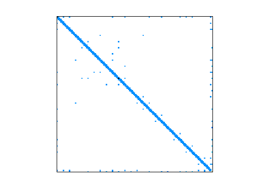
Matrix: Rommes/S40PI_n1
Description: Transmission line, 40 sections, SISO, index-1 DAE (CEPEL, Brazil)
|
| (undirected graph drawing) |
 |
 |
 |
| Matrix properties | |
| number of rows | 2,028 |
| number of columns | 2,028 |
| nonzeros | 5,007 |
| structural full rank? | no |
| structural rank | 2,025 |
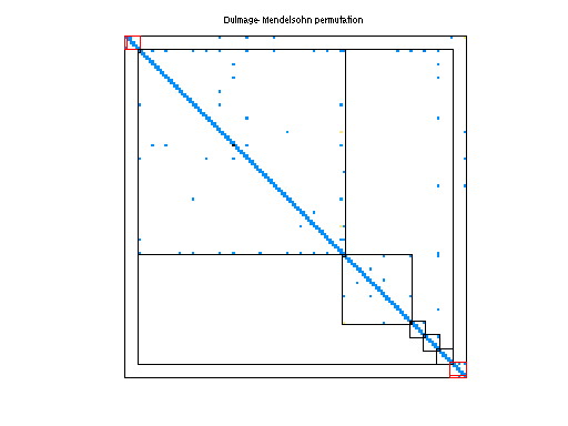
| # of blocks from dmperm | 23 |
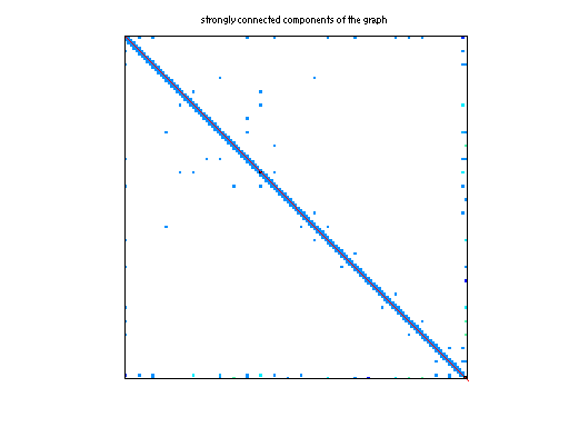
| # strongly connected comp. | 3 |
| explicit zero entries | 0 |
| nonzero pattern symmetry | symmetric |
| numeric value symmetry | 0% |
| type | real |
| structure | unsymmetric |
| Cholesky candidate? | no |
| positive definite? | no |
| author | F. Freitas |
| editor | J. Rommes |
| date | 2010 |
| kind | eigenvalue/model reduction problem |
| 2D/3D problem? | yes |
| Additional fields | size and type |
| B | sparse 2028-by-1 |
| C | sparse 1-by-2028 |
| E | sparse 2028-by-2028 |
Notes:
Power system models from Joost Rommes, Nelson Martins, Francisco Freitas

This collection of power system models originates from real power systems,
mostly based on Brazilian interconection power systems (BIPS) models (the file
names refer to the actual power system related to a given year electric load
scenario).  These systems [E dx/dt = Ax + Bu ; y=Cx + Du] are interesting
benchmarks for several numerical algorithms, including eigenvalue algorithms
(dominant modes/poles/zeros, stability analysis, computing rightmost
eigenvalues and/or with smallest damping ratio, eigenvalue parameter
sensitivity) and model order reduction (large-scale DAEs ). Refer to the
corresponding publications for more details on the systems and numerical
results of several eigenvalue/model order reduction algorithms. For
corresponding software, see http://sites.google.com/site/rommes/software

If E is not present in the problem, then E=I should be assumed.
If D is not present, D=0 should be assumed.  (Note that as of Jan 2011,
no problem has a nonzero D).

The iv vector in some of the files is a vector with nonzeros (ones) at indices
that represent state-variables (the zeros are algebraic variables). One can
construct the descriptor matrix E by E=spdiags(iv,0,n,n). This iv vector is
generated by the Brazilian power system simulation software, and can be more
efficient to compute with.

Test systems:

All power system models originate from CEPEL ( http://www.cepel.br/ )

power system    file                    n  #inputs #outputs  references
------------    ----               ------  ------- --------  --
New England     ww_36_pmec_36          66   1       1        [1]
BIPS/97         ww_vref_6405        13251   1       1        [1]
BIPS/2007       xingo_afonso_itaipu 13250   1       1        [2]
BIPS/97         mimo8x8_system      13309   8       8        [3]
BIPS/97         mimo28x28_system    13251  28      28        [3]
BIPS/97         mimo46x46_system    13250  46      46        [4]
Juba5723        juba40k             40337   2       1        [5]
Bauru5727       bauru5727           40366   2       2        [5]
zeros_nopss     zeros_nopss_13k     13296  46      46        [5]
xingo6u         descriptor_xingo6u  20738   1       6        [5]
nopss           nopss_11k           11685   1       1        [5]
xingo3012       xingo3012           20944   2       2        [5]
bips98_606      bips98_606           7135   4       4        [6]
bips98_1142     bips98_1142          9735   4       4        [6]
bips98_1450     bips98_1450         11305   4       4        [6]
bips07_1693     bips07_1693         13275   4       4        [6]
bips07_1998     bips07_1998         15066   4       4        [6]
bips07_2476     bips07_2476         16861   4       4        [6]
bips07_3078     bips07_3078         21128   4       4        [6]

Several SISO/MIMO test systems, whose main components are transmission lines
(TL) are available.  TLs are modeled by ladder networks, comprised of cascaded
RLC PI-circuits, having fixed parameters.

   Transmission lines with 10--80 PI Sections are considered.
   PIsections10to80.zip            [Submitted]

   There are two kinds of files for representing a same system: the file with
   termination _n refers to an index-2 system DAE model, while _n1 means
   a model of the same system, but for an index-1 DAE representation.  The
   representation of each test system has the form [E dx/dt = Ax + Bu ; y=Cx]

References:

[1] ROMMES, J., MARTINS, N., Efficient computation of transfer function
    dominant poles using subspace acceleration.  IEEE Trans. on Power Systems,
    Vol.  21, Issue 3, Aug. 2006, pp. 1218-1226

[2] ROMMES, J., MARTINS, N., Computing large-scale system eigenvalues most
    sensitive to parameter changes, with applications to power system
    small-signal stability , IEEE Transactions on Power Systems, Vol. 23, Issue
    2, May 2008, pp.  434-442

[3] ROMMES, J., MARTINS, N., Efficient computation of multivariable transfer
    function dominant poles using subspace acceleration.  2006, IEEE Trans. on,
    Power Systems, Vol. 21, Issue 4, Nov. 2006, pp.  1471-1483.

[4] MARTINS, N., PELLANDA, P.C.,ROMMES, J., Computation of transfer function
    dominant zeros with applications to oscillation damping control of large
    power systems, IEEE Trans. on Power Systems, Vol. 22, Issue 4, Nov. 2007,
    pp.  1657-1664

[5] ROMMES, J., MARTINS, N., FREITAS, F., Computing Rightmost Eigenvalues for
    Small-Signal Stability Assessment of Large-Scale Power Systems, IEEE
    Transactions on Power Systems, Vol. 25, Issue 2, May 2010, pp.929-938

[6] FREITAS, F., ROMMES, J., MARTINS, N., Gramian-Based Reduction Method
    Applied to Large Sparse Power System Descriptor Models, IEEE Transactions
    on Power Systems, Vol. 23, Issue 3, August 2008, pp. 1258-1270
| Ordering statistics: | result |
| nnz(chol(P*(A+A'+s*I)*P')) with AMD | 5,659 |
| Cholesky flop count | 1.6e+04 |
| nnz(L+U), no partial pivoting, with AMD | 9,290 |
| nnz(V) for QR, upper bound nnz(L) for LU, with COLAMD | 5,595 |
| nnz(R) for QR, upper bound nnz(U) for LU, with COLAMD | 9,041 |
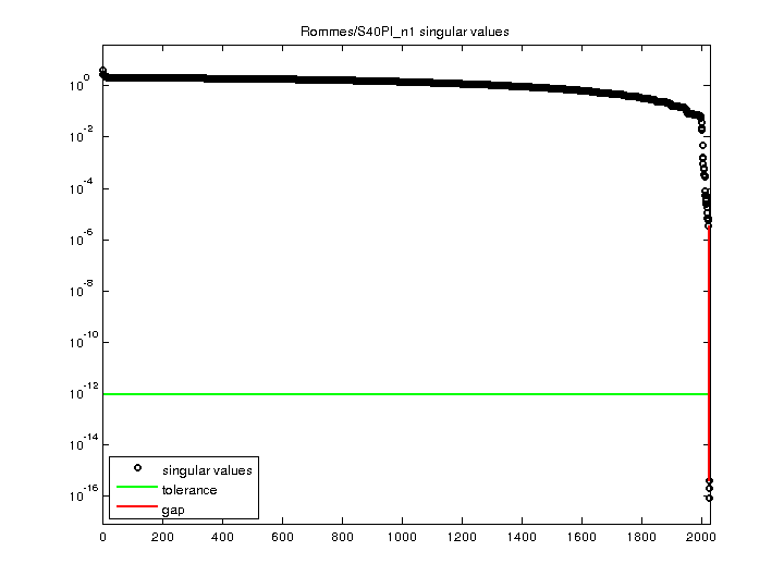
| SVD-based statistics: | |
| norm(A) | 3.97881 |
| min(svd(A)) | 8.65107e-17 |
| cond(A) | 4.59922e+16 |
| rank(A) | 2,025 |
| sprank(A)-rank(A) | 0 |
| null space dimension | 3 |
| full numerical rank? | no |
| singular value gap | 8.32306e+09 |
| singular values (MAT file): | click here |
| SVD method used: | s = svd (full (A)) ; |
| status: | ok |
For a description of the statistics displayed above, click here.
Maintained by Tim Davis, last updated 12-Mar-2014.
Matrix pictures by cspy, a MATLAB function in the CSparse package.
Matrix graphs by Yifan Hu, AT&T Labs Visualization Group.