Data Structures, Algorithms, & Applications in C++
Chapter 21, Exercise 2

(a)

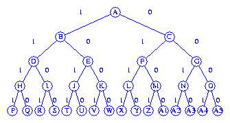
The tree is obtained from Figure 20.2 by adding an additional level with 16 nodes. The edge labels for the new edges represent values of x4 The new tree is given below.

(b)

The FIFO branch-and-bound search traverses the trees by levels and within levels left to right. Infeasible nodes are eliminated and their children are not generated.

We begin with node A as the E node. Its children B and C are feasible and added to the queue of live nodes. The next E node is node B. Its children, nodes D and E are generated. Nodes D and E are feasible and so are added to the queue. The next E node is node C. Both its children are feasible and so both are added to the queue. D becomes the new E node and its two children H and I added to the live node queue. Next nodes J, K, L, M, N, and O are added to the queue. Following this, node H becomes the E node. Its left child is infeasible. Its right child Q is a fesible leaf with value 9. This is the best leaf found so far.

When I is the E node, nodes R and S are generated. Node R is infeasible and S is a leaf with smaller value than Q. The next E node is node J. Its left child is infeasible and its right child is a leaf with smaller value than Q. Although both children of K are feasible, neither is better than Q. L, M, N, and O are the next four E nodes. Neither leads to a better leaf than Q. The live node list becomes empty and the search terminates with node Q as the best leaf.

(c)

The objects are already in nonincreasing order of profit density. So no rearrangement is necessary. Applying the bounding function at the root, we obtain 9 as an upper bound on the optimal filling. (Actually, since the bounding function has an all integer solution (1,1,1,0), this solution is optimal for the 0/1 knapsack and we can stop right away. In the following, we assume that we did not make this observation.)

We start with node A as the E node. Node B has value 4 and node C has value 0. Both nodes are added to the queue. Node B is expanded to get nodes D and E. The value of D is 7. The upper bound at E is 4 + 2 + 1/2 < 7. So E is not added to the live node queue. C is the next E node. The upper bound at its left child F is 3 + 2 + 1/4 < 7. So F is discarded. The bound at G is 2 + 3/4. So G is also discarded. The remaining live node D becomes the E node. Its left child has value 9, which equals the upper bound. So we can terminate. The nodes generated are A, B, C, D, E, F, G, and H. From H we can obtain the solution by setting the remaining xis to zero.

(d)

When a maximum-profit branch and bound is used, A is the first E node. Its children B and C are placed into a max priority queue. The value of B is 4 and that of C is 0. B is the next E node and its children D and E are added to the priority queue. Their vaues are 6 and 4, respectively. D is the next E node. Its children Hand I are added to the priority queue. Their values are 9 and 6. H becomes the next E node. Its left child is infeasible and its right child represents the best solution found so far. Nodes are extracted from the priority queue until the queue becomes empty. Upon termination, Q represents the best solution.

(e)

Using the bounding function of (c), we begin as in (d). After B and C are added to the Q, B becomes the E node as it has the best bound, 9. B's children are generated. D has value 7. The bound for E is less than 7. So E is discarded. The bound for D is maximum (9) and D is the next E node. Its left child H has value 9 and its right child has value less than this. H becomes the next E node. Since its value equals the upper bound, the search terminates.