Matrix: Sinclair/3Dspectralwave
Description: 3-D spectral-element elastic wave modelling in freq. domain, C. Sinclair, Univ. Adelaide
|
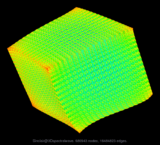
| (undirected graph drawing) |
 |
| Matrix properties | |
| number of rows | 680,943 |
| number of columns | 680,943 |
| nonzeros | 30,290,827 |
| structural full rank? | yes |
| structural rank | 680,943 |
| # of blocks from dmperm | 1 |
| # strongly connected comp. | 1 |
| explicit zero entries | 3,359,762 |
| nonzero pattern symmetry | symmetric |
| numeric value symmetry | symmetric |
| type | complex |
| structure | Hermitian |
| Cholesky candidate? | yes |
| positive definite? | no |
| author | C. Sinclair |
| editor | T. Davis |
| date | 2007 |
| kind | materials problem |
| 2D/3D problem? | yes |
| Additional fields | size and type |
| b | sparse 680943-by-1 |
| shift | sparse 680943-by-680943 |
Notes:
The A matrix is produced using 3-D spectral-element elastic wave modelling in
the frequency domain. The medium is homogeneous and isotropic with elastic
coefficients: c11 = 6.30,  c44 = 1.00 The B matrix represents a real
y-directed source, placed approximately in the centre.  The model size in
elements is 20x20x20. Each element is 1m x1m x 1m. Each element is a 4x4x4
Gauss-Lobbato-Legendre mesh, so the height, width and depth of the system is
61 nodes. There are 3 unknown components at each node - the x, y and z
displacements. The A matrix therefore has dimension 680943 x 680943, where
((20 x 4) - (20 - 1))^3 * 3 = 680943. The problem domain is earth sciences.
Note that A is complex and b is sparse and real (b has a single nonzero).

The A matrix was provided with a nonzero imaginary part, but was otherwise
complex Hermitian.  To save space in the Matrix Market and Rutherford/Boeing
formats, the A matrix here has had this imaginary diagonal removed.  The
shift can be found in the aux.shift auxiliary matrix.  To reproduce the
original A matrix, use A = Problem.A + Problem.aux.shift ;
| Ordering statistics: | result |
| nnz(chol(P*(A+A'+s*I)*P')) with AMD | 9,565,680,684 |
| Cholesky flop count | 4.3e+14 |
| nnz(L+U), no partial pivoting, with AMD | 19,130,680,425 |
| nnz(V) for QR, upper bound nnz(L) for LU, with COLAMD | 16,486,249,140 |
| nnz(R) for QR, upper bound nnz(U) for LU, with COLAMD | 34,447,602,838 |
Note that all matrix statistics (except nonzero pattern symmetry) exclude the 3359762 explicit zero entries.
For a description of the statistics displayed above, click here.
Maintained by Tim Davis, last updated 12-Mar-2014.
Matrix pictures by cspy, a MATLAB function in the CSparse package.
Matrix graphs by Yifan Hu, AT&T Labs Visualization Group.